A Computation Fluid Dynamics Methodology for the Analysis of the Slipper–Swash Plate Dynamic Interaction in Axial Piston Pumps

Abstract

This paper proposes a CFD methodology for the simulation of the slipper’s dynamics of a swash-plate axial piston unit under actual operating conditions. The study considers a typical slipper design, including a vented groove at the swash-plate interface. The dynamic fluid–body interaction (DFBI) model is exploited to find the instantaneous position of the slipper, while the morphing approach is adopted to cope with the corresponding mesh distortion. A modular approach is adopted to ensure high-quality mesh on the entire slipper surface and sliding interfaces provide the fluid dynamic connection between neighboring regions. The external forces acting on the slipper are included by means of user-defined lookup tables with the simulation estimating the lift force induced by fluid compression. Moreover, the force produced by the metal-to-metal contact between the slipper and the swash plate is modeled through a specific tool of the software. The pressure signal over an entire revolution of the pump is taken as an input of the simulation and a variable time step is used to manage the high-pressure gradients occurring in the regions of inner and outer dead points of the piston. The weakly compressible characteristic of the fluid is considered by a specific pressure-dependent density approach, and the two-equation eddy-viscosity k-ω SST (shear stress transport) model is used to assess the turbulent behavior of the flow. Furthermore, the transitional model predicts the onset of transition, thus solving different equations depending on whether the flow enters a laminar or turbulent regime. In conclusion, the proposed methodology investigates the motion of the slipper in response to several external forces acting on the component. The numerical results are discussed in terms of variable clearance height, pressure distribution within the gap, and lift forces acting on the slipper under specific pump operations.

1. Introduction

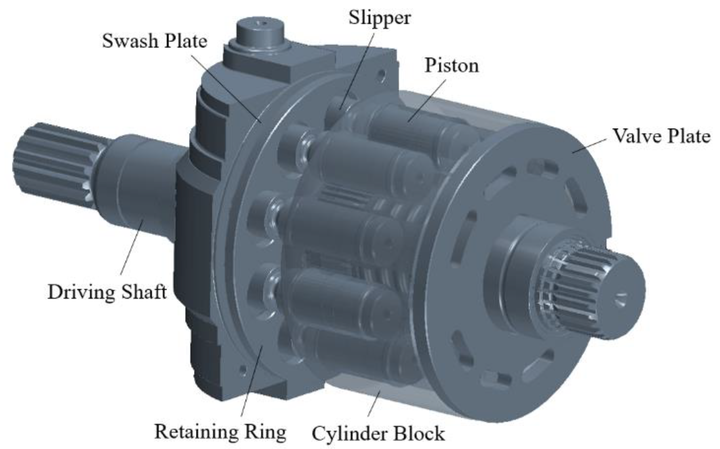
Within the wide range of positive-displacement machines commonly used in industrial and mobile applications, piston pumps and motors are recognized worldwide as the most sophisticated ones. The high number of internal components along with the advanced working principle require fine mechanical couplings and a precise phasing of the moving parts, proves necessary to ensure the proper machine’s operation. Nowadays, swash-plate-type axial piston pumps represent the most frequent choice for many users due to the extremely consolidated technology, which yields very high efficiencies at critical operating pressures, up to 400 bar. On the other hand, very fine machining tolerances and surface roughness are needed to reach the best possible pump performance. At the same time, the huge number of components leads to a high cost and weight compared to other positive-displacement machines, which still represent the main demerits for such architecture. The layout of a commercial swash-plate axial piston pump is presented in Figure 1.

In this case, the roto-translating motion of nine pistons arranged at a constant angular distance from each other is exploited to transfer the operating fluid from the low-pressure side, namely the suction port, to the high-pressure environment, namely the supply port. The continuous connection between the displacement chambers with both sides of the pump is achieved typically through a plane valve plate. In detail, considering an entire piston revolution, the expansion produced by the piston stroke from the inner dead point (IDP) to the outer dead point (ODP) generates a local depression, which draws fluid from the suction port, while the reversed piston stroke, i.e., from the ODP to the IDP, forces the fluid through the supply port by means of local compression. The cylinder block hosts the pistons’ stroke within nine cylindrical seats and a direct connection of the cylinder block with the primary shaft of the pump ensures the rotation of the entire group.

On the other hand, the pistons’ stroke depends on the swash-plate inclination angle, which further determines the pump displacement. Nowadays, the mechanical coupling between pistons and the swash plate is mainly realized through the slippers, which prevent the relief of the contact between parts at the cost of an additional moving element for each piston of the pump. These few lines only aim to offer the reader an overview of the swash-plate axial piston pump working principle, but an extremely exhaustive description of the complex mechanism of these machines can be found in [1].

This paper focuses on the analysis of the slipper–swash plate dynamic interface, whose design strongly influences the overall efficiency of the pump, both in terms of volumetric and mechanical losses. The slipper accommodates the piston rotation by sliding on the flat surface of the swash plate while preserving the components integrity, and a net pushing force pressing the slipper towards the swash plate is generated. The metal-to-metal contact between parts is mitigated by a thin layer of fluid amongst the mating surfaces, which supports the slipper though hydrostatic and hydrodynamic lift. Therefore, the clearance height represents a crucial parameter in the pump design as it should minimize leakages while avoiding friction produced by the mechanical contact between components. Moreover, from a microscopic point of view, the slipper undergoes almost imperceptible tilting motions, which slightly influence the gap internal fluid dynamics, thus producing instantaneous variations in the clearance height that require highly advanced analysis to be assessed. For this reason, a great effort has been made in the last few decades to optimize the slipper–swash plate group with remarkable effects on the hydrodynamic efficiency of these pumps.

A power-loss model of the slipper–swash plate pair, including the slipper deformation, is presented in [2]. The results highlight a major effect of the slipper rotational velocity on the overall power losses, while the external operating pressure only produces secondary effects. Moreover, the influence and impact of the gap between the outer and the inner diameter of the slipper on the performance of axial piston pumps is studied in [3]. In this work, the authors investigated the optimum fluid film thickness, which minimizes the power losses between the slipper and the swash plate for different slipper designs. A designing procedure whereby the slipper behavior, minimum film thickness, and flow losses can be estimated is further outlined in [4]. It is shown that for successful operation, the slippers require a small amount of non-flatness on the running surfaces. Additionally, the authors pointed out the difficulties in building a proper test rig that can precisely reproduce the real slipper behavior within the pump. For this reason, some approximations must always be made. In this case, the proposed test rig allows the slipper under steady-state conditions to be investigated, and the rotating motion is here assigned to the swash plate instead of the slipper to remove centrifugal effects. The test rig was finally validated through results comparison with the theoretical predictions. Exploring the literature, the most advanced test rig configuration for the experimental analysis of slipper–swash plate coupling is presented by Zhang et al. in [5]. It consists of a redesigned three-piston pump that minimizes the alterations to the original component where the reduced number of pistons helps to address the potential space limitation of the sensors’ installation.

As reported in [4], minimal details, such as the surfaces’ shape and materials, can significantly affect the overall efficiency of the pump. This concept is further stressed in [6], in which different experimental measurements highlight the benefits of an appropriate nanocoating applied to the slippers surface in reducing friction losses.

Along with the experimental approach, the analytical method still represents a practical tool for the analysis of slipper fluid dynamics. In [7], the Reynolds equation for slipper bearing considering the entire slipper dynamics is obtained and accurately discussed.

In recent years, the increasing computational power of modern computers has led to the implementation of several numerical tools, which have assisted researchers in deeply understanding and optimizing the internal behavior of the many pump components, including the slipper–swash plate pair. In [8], Wieczorek and Ivantysynova presented one of the most advanced simulation tools for swash-plate-type axial piston pumps, i.e., CASPAR. The numerical model determines the instantaneous gap heights by continuously solving the motion equation for all moveable parts of the rotating group. This yields the calculation of the main losses generated in the machine due to viscous friction and gap flow. The CASPAR method has been continuously improved and further exploited over the years since the latest work was described in [9], in which the effect of the ball socket joint on the shear and volumetric losses through both the slipper–swash plate and piston–cylinder interfaces is investigated. In [10], the results of dynamic contact analysis of the piston–slipper pair highlight the effects of piston radius enlargement, as well as of a radial clearance reduction in improving the normal displacement, the maximum contact pressure, the contact radius, and the normal and tangential contact stiffness.

Three-dimensional numerical models certainly represent the largest source of information in product design as they predict the physical variables’ distribution over the entire 3D domain under actual operating conditions, thus facilitating the identification of any critical issues before prototyping. Furthermore, these specific tools allow designers to explore a greater number of possibilities while making quick and efficient revisions. A relevant example for that is reported in [11], in which a practical and effective use of the CFD methods is shown regarding the influence of hydrodynamic processes on fluid flow characteristics following the installation of angular fitting connections in pipeline systems. For this reason, three-dimensional simulations are now also firmly included in the design process of axial piston pumps and motors. In [12], a finite element method (FEM) model is implemented to evaluate the stresses, strains, and forces associated with the crimping process used in piston–slipper coupling, while a computational fluid dynamics (CFD) methodology for the simulation of an entire swash-plate axial piston pump, including nominal leakages, is proposed in [13]. A detailed comparison between lumped parameters and computational fluid dynamics (CFD) approaches for the simulation of axial piston pumps is presented in [14,15]. The importance of 3D tools for the optimization of detailed features and fine-tuning has been highlighted. In [16], a multiphase CFD approach is exploited to predict the heat transfer between moving metal parts and oil within a piston water pump, and a lumped parameters model of the whole machine is implemented.

Lately, promising results have also been reached with the help of the latest generation of computational technologies. In [17], a neural network approach is used to investigate the effect of several design parameters on slipper performance. A good agreement with experimental data shows the capability of the proposed methodology in analyzing actual bearing systems.

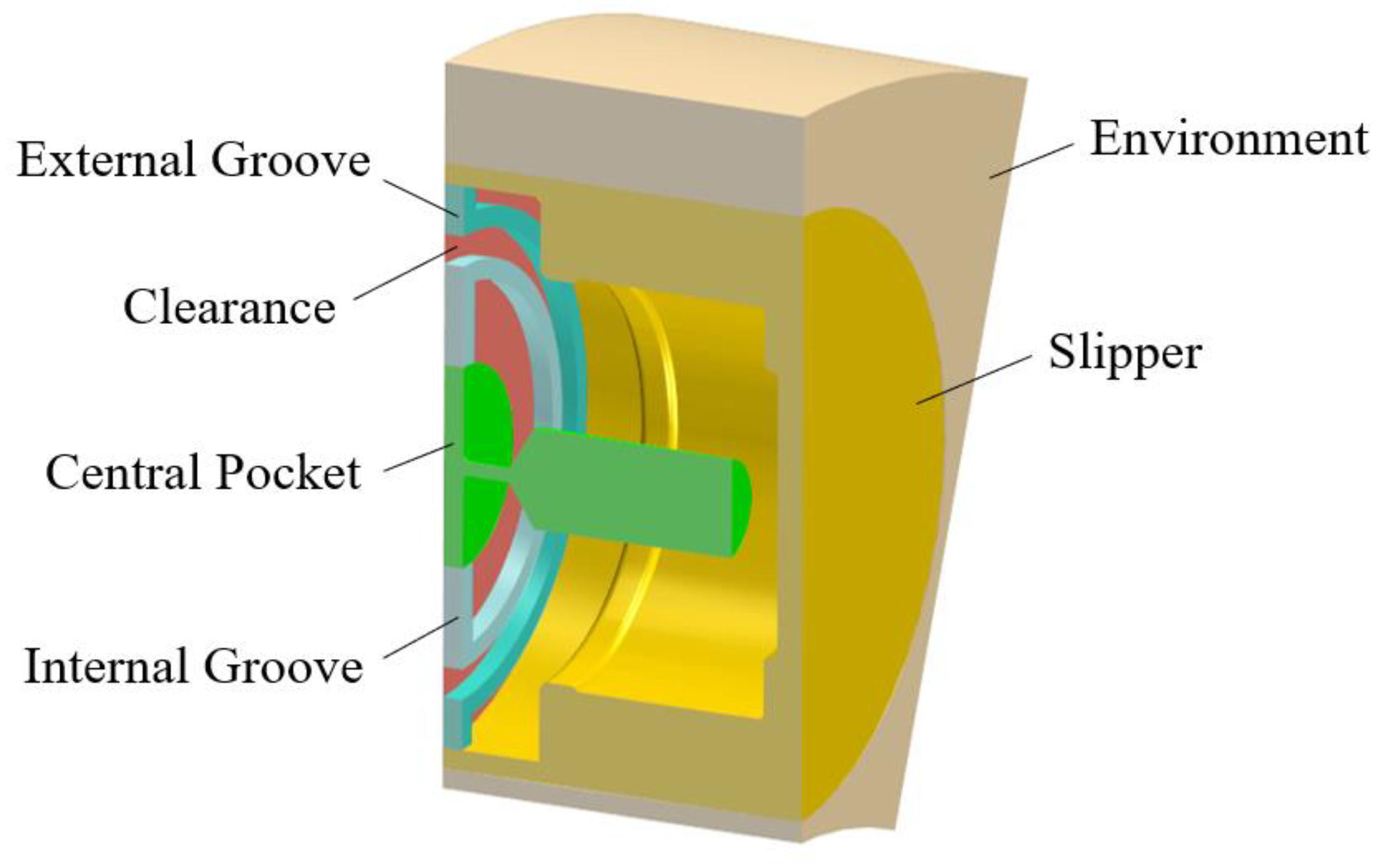
Several slipper architectures have been developed over the years to progressively reduce volumetric and power losses within axial piston machines. Currently, three main slipper designs can be found in industrial pumps and motors, each one characterized by its own advantages and disadvantages.

• Single-land slipper: it represents the original slipper design. It shows a single pocket at the center of the slipper sliding surface, directly connected to the main pressure source through the slipper hole. This design ensures the minimum possible leakage flow through slipper–swash plate clearance;
• Grooved slipper: one or more circular grooves are obtained on the running surface of the slipper. This device brings much more stability to the slipper as it periodically switches from a high-tilt position to a nearly flat one over each revolution of the pump. In this case, the leakage flow is always increased with respect to the single-land configuration, while the lift force may increase or decrease depending on the groove position central radius according to [18];
• Vented grooved slipper: the more external groove is connected to the drain pressure through one or more radial connections with the intention of reducing the slipper spin. However, in this configuration, the external groove does not produce hydrostatic lift, thus leading to a significant reduction in the lift force with respect to both previous designs.

The three slipper designs are reported in Figure 2 for a real commercial component.

In [19], an explicit approach to determine the general flow and pressure drop equations for a multiple-land slipper is proposed. For this study, a real slipper geometry, including a single balancing groove, was considered. In [20], a comparison between a grooved slipper and a single-land slipper was performed in terms of pressure distribution, flow losses, and lift forces for both configurations. The huge weight of the groove position and length on the slipper lift force was outlined since an increase or even a decrease in the lift force versus the single-land slipper was observed depending on the geometrical features of the groove. Moreover, this paper includes a CFD simulation of the slipper at a specific tilt angle to evaluate the flow and pressure distribution through the gap. However, no slipper dynamics are considered, and a fixed mesh is used.

This manuscript proposes for the first time a fully CFD methodology that is able to predict and simulate the dynamics of a slipper in axial piston pumps under actual operating conditions. The slipper design considered in this paper is a vented grooved slipper as shown in Figure 2c. The three-dimensional CFD model accounts for the fluid–body interaction to instantly update the slipper position as a result of the variable force balance acting on the component, thus showing the effects on both micro-motion intensity and the variable clearance height by means of deformable mesh techniques. The slipper–swash plate contact is further handled by the solver through a particular tool of the software, which allows the separate contribution of both the hydraulic force and the contact force to be evaluated.

2. Materials and Methods

The CFD analysis presented in this paper was performed through the multi-purpose STAR-CCM+ v.2021.1.1 platform, licensed by Siemens [21]. The advanced CAD tools embedded in the software were used to extract the three-dimensional fluid domain as a set of separate adjacent regions, thus meeting the principles of modularity. In effect, a modular approach was adopted to facilitate the generation of a high-quality mesh near the slipper’s surfaces, which proved necessary for such a demanding application. From a geometrical point of view, this study focused on a 40-degree circular sector associated with a single slipper of a reference nine-piston pump. The piston geometry was neglected as it would have introduced even more modeling problems without substantially changing the accuracy of the results. Nevertheless, the footprint of the piston cap within the slipper’s spherical socket was included to address the piston–slipper ball joint. Moreover, according to practical measurements performed on the real component, an initial clearance height h₀ was considered between the slipper and the swash plate. In Figure 3, a section view of the entire computational domain highlights the fluid regions associated with the main elements of the slipper.

The fluid domain discretization certainly represented the most challenging phase in the model setup since an extremely high-quality mesh was needed to cope with the instantaneous cells’ distortion produced by the slipper motion. Consequently, a refined mesh was created near the slipper walls by means of local surface controls, and remarkable care was devoted to the geometrical discretization of the slipper–swash plate interface, including both the grooves and the leakage region. In detail, an automated polyhedral mesh was adopted within the entire fluid domain, except for the clearance where a butterfly grid was exploited, [22]. In

Table 1. Mesh size.

Fluid Regions	Cell Shape	Base Size
Central pocket	Polyhedral	16.7h0
Grooves	Polyhedral	6.7h0
Slipper	Polyhedral	16.7h0
Environment	Polyhedral	33.3h0

, the base size associated with the different fluid regions is reported as a function of the design parameter h₀.

Moreover, a local cell size of 3.33h₀ was forced at the interfaces with the gap, and two boundary layers were generated near the solid surfaces. The extruded mesh approach was used for the axial discretization of regular-shape volumes, such as the leakage and the grooves, where five and fifteen cell layers were respectively defined. Ultimately, the three-dimensional grid resulted in almost 3.4 million cells, corresponding to a 14-day computational time on a modern cluster architecture with 160 processors for the simulation of an entire revolution of the shaft. In Figure 4a, a central section of the slipper highlights the fluid domain discretization, while two separate views of the mesh within the slipper pocket and inside grooves are shown in Figure 4b,c, respectively. In Figure 4d, a very expanded view of the mesh within the gap reveals the 0.2h₀ layers’ height.

The many fluid regions were coupled through standard in-place interfaces, while a 40-degree periodic interface was set at both sides of the domain to include the effect of the adjacent slippers on the internal fluid dynamics.

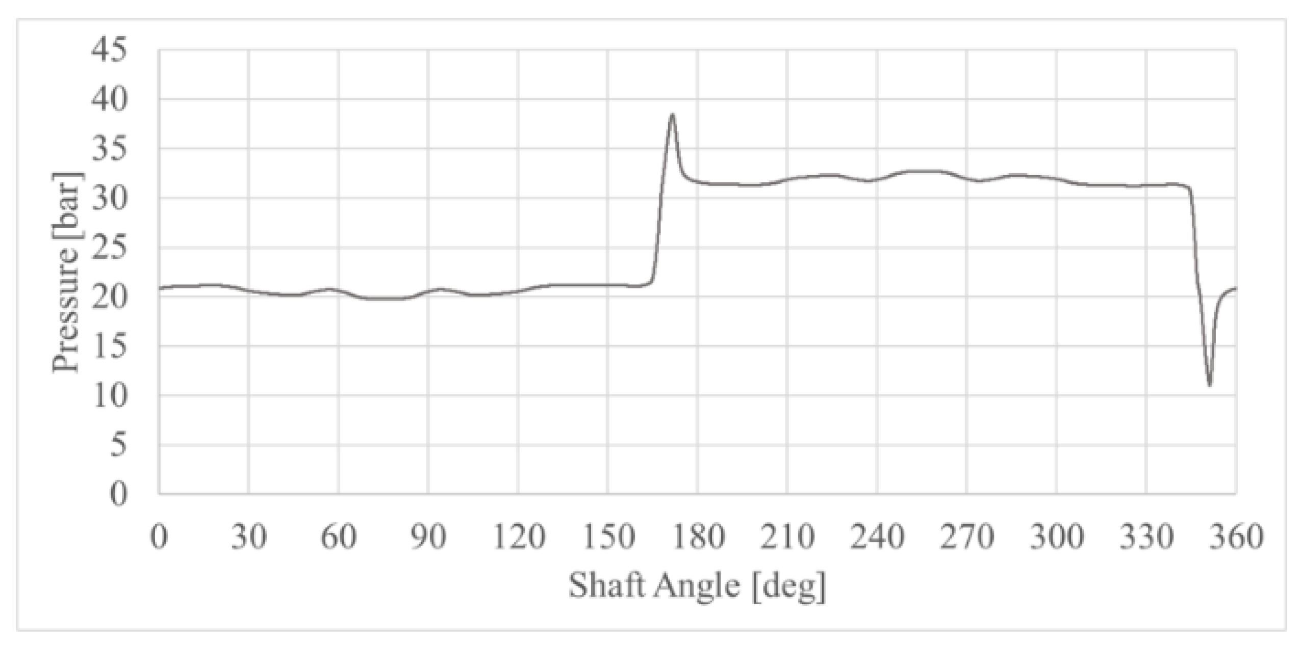
The proposed numerical methodology was tested at a specific pump-operating condition extracted from a real closed-circuit application in off-highway vehicles. A schematic representation of the simulated working point is reported in

Table 2. Simulated operating conditions.

Parameter	Symbol	Value
Rotational speed	npump	2500 rpm
Swash-plate inclination angle	β	18 degrees
Supply pressure	pout	30 bar
Suction pressure	pin	20 bar
Drain pressure	pdrain	0.5 bar

. The instantaneous pressure signal within the slipper central pocket was derived by combining the results of a previously validated 0D–1D model of the entire pump with the dynamic CFD analysis presented in [13]. The pressure data were sampled every 0.06 degrees of shaft rotation, and they were further included in the CFD model through imported tables and user-defined field functions, thus obtaining the inlet pressure curve displayed in Figure 5. In parallel, the drain pressure was set at the outer region by means of constant pressure outlets.

In terms of motions, the revolution of the slipper around the primary shaft of the pump was not directly assigned to the fluid domain. Indeed, the original position of the external boundaries was fixed over the entire simulation period, while the wall tangential velocity associated with the pump rotational speed was forced on the surfaces of the slipper. Consequently, this kind of approach did not address the centrifugal force produced by the slipper rotation, which required external implementation by the user. For this reason, the definition of the external forces acting on the slipper is accurately treated in the next paragraphs.

The rigid body assumption was made for the slipper and the dynamic fluid–body interaction (DFBI) tool was used to predict the slipper motion according to the many forces acting on it. Indeed, the proposed method allows the motion of a rigid body to be simulated in response to forces exerted by the fluid, or to any additional external forces provided by the user, while the internal algorithm solves the governing equations of motion to find the new position of the object. In Figure 6, the three-dimensional free-body diagram of the slipper highlights the separate contributions of both mechanical and hydraulic forces causing the characteristic micro-motions of the component. In this context, referring to the barycentric coordinate system shown in Figure 6, the slipper was modeled as a three-DOF (degrees of freedom) body with the possibility of undergoing rotations about both the X-axis and the Y-axis, as well as translating along the Z-axis. For this reason, the multi-body motion DFBI model was selected to address the specific application involving two rotational degrees of freedom.

As accurately explained in [1], the mainly axial pressure-dependent force F_pi,i produced by the pressurization of the piston effective area is further transmitted to the slipper through the piston–slipper ball joint as in (1):

$${\mathrm{F}}_{\mathrm{pi},\mathrm{i}-\mathrm{sl},\mathrm{i}}=\frac{{\mathrm{F}}_{\mathrm{pi},\mathrm{i}}}{\cos \mathsf{\beta }},$$

(1)

F_pi,i-sl,i represents the net piston force pressing the slipper towards the swash plate, while β symbolizes the swash-plate inclination angle. Moreover, the constraint force produced by the slippers retaining ring F_rp-sl,i and the centrifugal force generated by slipper rotation F_sl,icen were added to the model in the form of external forces acting on the rigid body. On the other hand, the weight F_sl,ig, the force of inertia F_sl,iI, the viscous friction force F_sl,ivisc, and the contact force F_sw-sl,i produced by the slipper–swash plate collision were all included in the results of the simulation. In particular, the weight contribution was computed from the gravity acceleration included in the continuum properties along with the peculiar mass of the slipper. The lumped parameters model of the full pump was exploited to derive the evolution of the external forces as a function of the slipper angular position φ. The resulting dataset was imported in the CFD simulation through bi-dimensional file tables, while the corresponding plots were normalized with respect to the maximum force acting on the piston, F_pi,max, which are reported in Figure 7.

Moreover, three separate local reference systems with the same orientation were created at the forces’ origins to facilitate the definition of the external loads. Indeed, an accurate prediction of the slipper micro-motion cannot be separated from a detailed analysis of the active torques, which mainly depends on precise positioning of the forces’ application points.

The grid deformation produced by the slipper dynamics was addressed by means of the DFBI morphing technique, an advanced methodology of the software that displaces the mesh vertices according to the calculated motion of the rigid body without any computational-demanding remeshing processes. Despite its huge potential, the morphing approach requires an extremely high-quality initial mesh, and it brings a significant computational effort that implies long simulation periods. For this reason, a sophisticated modeling strategy was adopted to obtain reliable results in the shortest time possible. In detail, the modular approach was used to arbitrarily select the morphing regions, thus avoiding reckless use of this skill throughout the fluid domain. In effect, the morphing algorithm was only limited to the slipper outer walls where the cells’ vertices continuously change their relative position with respect to a fixed boundary, i.e., the swash plate and the interface with the environment. On the other hand, the fluid regions associated with the grooves and the slipper central pocket were forced to rigidly follow the motion of the DFBI body through an appropriate system of reports and superposing motions, thus constantly securing the connection with the deformable regions through variable interfaces. This shrewdness allowed the mesh distortion produced by the morpher to be minimized, thus avoiding the occurrence of negative volumes cells at any computational time step and preventing the simulation from aborting.

The main limitation of the morphing approach is that real contact between mating surfaces can never be reached as it would certainly produce zero or even negative volume cells. Therefore, a minimum gap between walls must always be kept in the mesh. This modeling specification introduced a practical issue in the simulation as the proposed slipper design expects permanent contact between parts to ensure adherence of the slipper to the swash plate, which represents the main requirement for a proper machine operation, according to the manufacturer. Consequently, a totally hydraulic lift of the slipper is not desired, and it must be avoided. That considered, a fictitious contact force was introduced by means of the contact coupling tool of the software. This force acts on the slipper in the swash-plate normal direction and it prevents the slipper’s surface from colliding with the swash-plate fixed boundary. The repulsive force linearly grows as the distance between parts decreases and it activates when the distance falls below a user-defined effective range, which was set to 0.33h₀ for this specific application. Furthermore, it is worth stressing that the spinning motion of the slipper, i.e., the revolution of the slipper about its own axis, was not addressed in this study as it would have produced high mesh distortions that are still not supported by the morphing methodology.

The physics continuum included an ISO VG 32 mineral oil [23], typically used in axial piston machines, and the fluid compressibility was considered as it significantly improves the predictive capability of the pumps’ CFD models [24]. The variation in fluid density ρ with respect to the working pressure p is shown in (2), where ρ₀ represents the fluid density at the atmospheric pressure, while c is the speed of sound of the oil.

$${\mathsf{{\rm P}}=\mathsf{\rho }}_0+\frac{\mathrm{p}}{{\mathrm{c}}^2},$$

(2)

The fluid properties were evaluated at the working temperature of 80 °C and an isothermal flow was assessed. In

Table 3. Properties of the oil for T = 80 °C.

Fluid Regions	Cell Shape	Base Size
Density at atmospheric pressure	ρ0	834 kg/m3
Dynamic viscosity	µ	8.14 mPa*s
Speed of sound	c	1300 m/s

, the specific parameters of the oil are summarized.

The evident time dependence of the investigated phenomenon required an implicit unsteady analysis. Moreover, a variable time step approach was adopted to cope with the strong pressure gradients occurring at the transition regions, i.e., when the piston switches from the suction side to the supply side and vice versa. Quantitatively, a time step of 4 µs corresponding to a 0.06-degree rotation of the driving shaft was used for both suction and supply intervals, while a temporal discretization of 1.33 µs proved necessary to ensure the numerical stability of the simulation during transitions.

The turbulent behavior of the flow was addressed by means of the two-equation K-Omega SST model [25,26], which blends the predictive capability of the K-Omega model within the boundary layer with the K-Epsilon-improved performance in the free-stream region. The all-y+ wall treatment was further selected to address a wide range of near-wall mesh sizes. This choice was confirmed by the low value of the wall y+ parameter, in the order of 0.1, within the most significative part of the domain, i.e., in the clearance region, due to the extremely short distance between the walls. In addition, the gamma transition model [27] was selected to predict the transitional flow throughout the three-dimensional domain, thus reaching a precise estimate of the fluid dynamics within the variable clearance between the slipper and the swash plate.

Finally, the conservation equations of mass and momentum were separately solved by means of the characteristic predictor–corrector approach of the segregated solver, and the SIMPLE algorithm was employed to control the solution update.

3. Results

In this section, the results of the proposed CFD analysis are reported, and the high predictive capability of the simulation is clearly pointed out throughout the text.

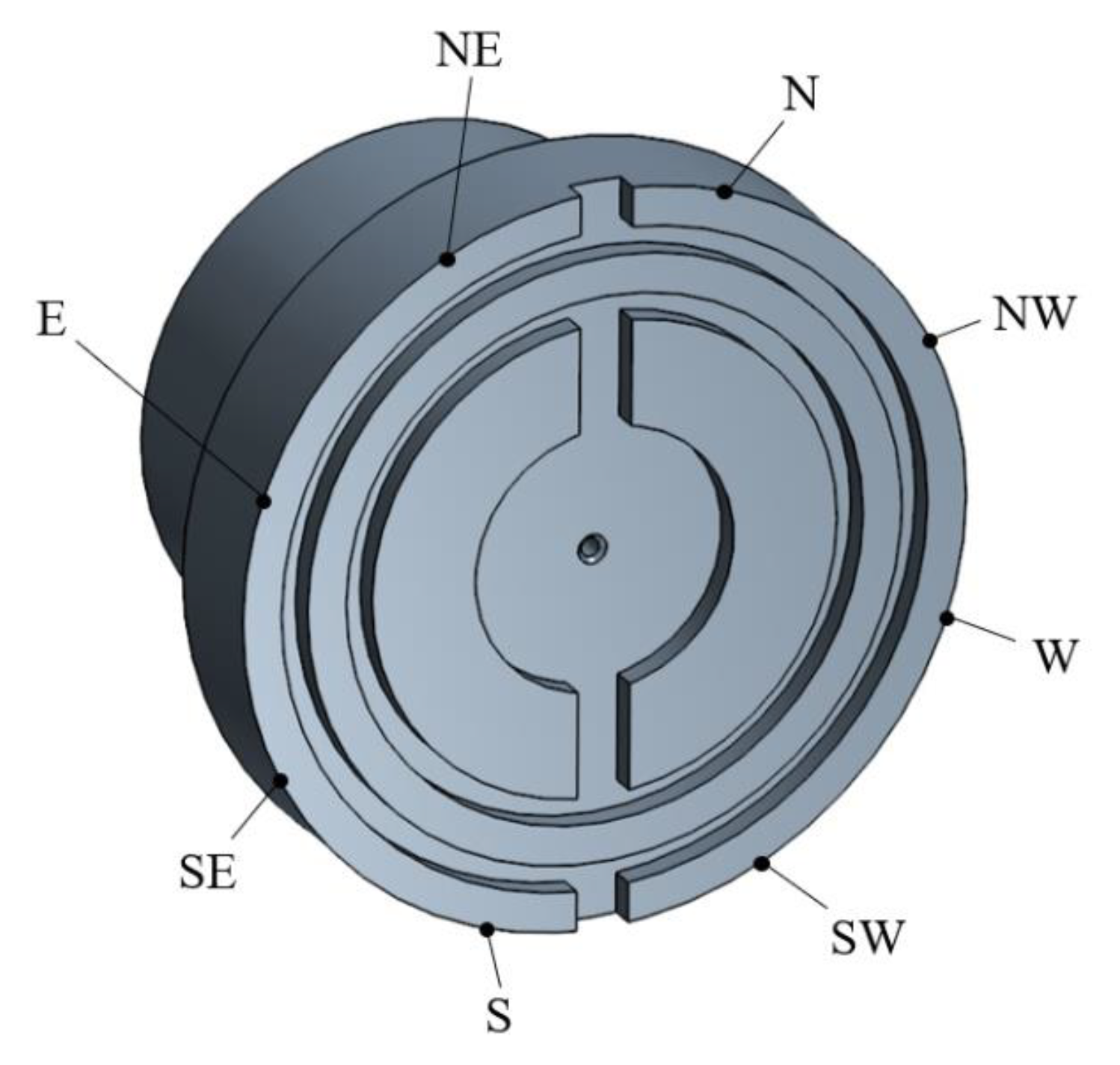
The reports manager node was exploited to predict the instantaneous position of the slipper, as well as to determine the corresponding minimum clearance height. The variable distance between the slipper and the swash plate was monitored through eight equally spaced cardinal points on the slipper’s sliding surface as shown in Figure 8. The rigid motion computed by the DFBI solver was further associated with the probes to update their positions according to the slipper motion. Therefore, the gap height was mapped over the entire slipper–swash plate interface as the instantaneous distance between the moving points and the fixed swash-plate boundary along the slipper axial direction, i.e., the Z-axis.

In Figure 9, eight different colors are used to outline the distance of each probe from the fixed swash-plate surface over a complete shaft revolution, therefore providing an effective description of the instantaneous slipper tilting under actual pump operations. The variation in the normalized clearance height during the first cycle of the pump is shown in Figure 9a. Starting from the nominal distance h₀, the slipper progressively moved towards the swash plate after reaching a dynamic equilibrium after a 25-degree initial transient. In Figure 9b, the same plot outlines the evolution of the slipper–swash plate distance over the second revolution of the driving shaft.

In detail, the periodic trend suggested the convergence of the simulation, and a minimum clearance height of 0.304h₀ was obtained at the suction-to-supply transition interval, during which the highest-pressure peak occurred. Moreover, in Figure 10, a zoomed view of the line integral convolution at the slipper outer radius gives a qualitative description of the gap maximum compression.

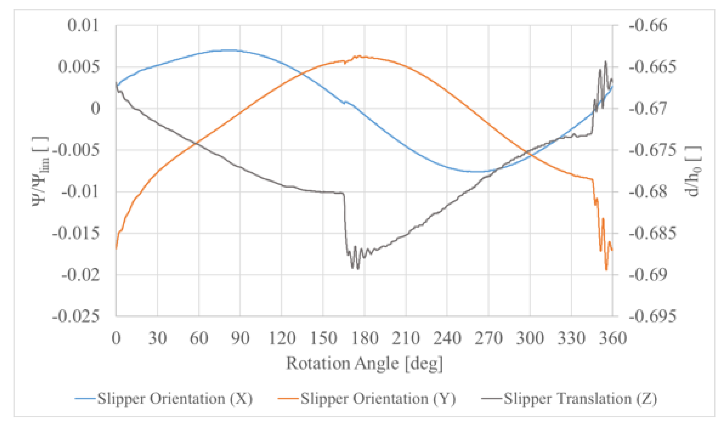
From now on, the proposed results only refer to the second revolution of the pump, thus excluding the initial spikes produced by the necessary numerical stabilization. In Figure 11, the separate contributions of the permitted rigid motions on the final position of the slipper are displayed in the normalized form. In detail, Ψ_lim represents the maximum tilt angle under nominal conditions, i.e., the angle Ψ, which produces slipper–swash plate contact for a central distance h₀ between parts. A sinusoidal trend was observed in the rotations about both the X-axis and the Y-axis, while a mainly linear characteristic interspersed with abrupt variations at the transition intervals was extracted for the slipper translation along the Z-axis. In absolute terms, the variable distance between the slipper and the swash plate is primarily influenced by the slipper axial displacement with a secondary effect produced by the tilting motions.

In terms of forces, Figure 12 highlights an almost constant hydraulic lift during both suction and supply intervals, while considerable spikes were observed at the transition regions. In detail, a mean force of 0.4F_pi,max was estimated over the suction period, while 0.62F_pi,max was measured at the supply phase due to the greater contribution of the hydrostatic lift. Moreover, a maximum force of 0.76F_pi,max was reached at the transition from the low-pressure to the high-pressure side of the pump, whereas an absolute minimum of 0.2F_pi,max was registered at the suction opening. On the other hand, the normalized repulsive force produced by the slipper–swash plate collision, which revealed specular behavior to that of the slipper translation, thus showing a linear increase in the contact force for the entire suction stroke followed by a descending ramp over the delivery phase. Once again, the occurrence of force peaks in the regions of outer and inner dead points of the piston were noted, where 0.4F_pi,max and 0.06F_pi,max forces were detected, respectively.

Furthermore, a dimensionless coefficient B_G was defined as in (3) to estimate the slipper hydraulic balancing:

$${\mathrm{F}}_{\mathrm{Gab}}{=\mathrm{B}}_{\mathrm{G}}·{\mathrm{F}}_{\mathrm{NS}},$$

(3)

In the equation, F_Gab represents the lift force acting on the slipper, whereas F_NS is the sum of the external forces pushing the slipper towards the swash plate. Therefore, three main conditions fully describe the instantaneous behavior of the slipper-swash plate interface.

• B_G < 1: the thrust force is not compensated by the lift component, thus suggesting slipper–swash plate contact. In this configuration, the contact force is enabled.
• B_G = 1: a perfect hydraulic balancing of the slipper is reached, thus preventing metal-to-metal contact between parts. Consequently, contact force does not apply in this case;
• B_G > 1: the lift contribution exceeds the thrust force, thus losing the fundamental coupling between the slipper and the swash plate.

As previously explained, the third situation must always be avoided since it causes a drastic reduction in the pump volumetric efficiency, which significantly affects the proper operation of the machine. For this reason, the slippers are typically designed to work with B_G < 1 and a certain slipper–swash plate contact is accepted.

In Figure 13, the balance coefficient is monitored on a full revolution of the pump and a sinusoidal trend in local discontinuities at the transition regions was observed. The signal denoted continuous adhesion of the slipper to the swash plate, and it further confirmed a greater imbalance of forces at the delivery port opening, where a minimum coefficient of 0.62 was reached.

At this point, it is worth specifying that the proposed results are clearly influenced by the 0.33h₀ effective range at which the contact force activates. Indeed, a more accurate prediction of the hydraulic force, as well as of the clearance height, would have required a reduction in the user-defined effective range. However, starting from h₀, this operation would have led to higher cells’ distortion with remarkable effects on the mesh stability. Therefore, the proposed solution is the best tradeoff between the results’ accuracy and the modeling limitations of the software.

In Figure 14, the leakage flow is reported as a percentage of the ideal flow rate delivered by the pump, Q_max, and it highlights the combined effect of both the working pressure and the clearance height. In effect, larger flow losses were measured at pump delivery due to the higher pressure drop across the gap, and a linear increase in the curve in this region was related to the progressive expansion of the flow area. A peak of 0.0079% was finally achieved before the complete closing of the outlet port, when the maximum flow area was reached over the entire supply interval. Instead, the minimum leakage was registered at the supply-to-suction transition, where the simultaneous presence of the lowest working pressure and the largest gap height produced an instantaneous flow rate equal to 0.0044% of Q_max. Hence, from the point of view of the volumetric losses at the slipper–swash plate interface for the proposed slipper design, this result emphasized a greater contribution of the inlet pressure with respect to the flow area.

In conclusion, the pressure drop through the gap was studied. In Figure 15, a 3D plot is used to map the pressure distribution at the slipper–swash plate interface during both suction and supply intervals, and a non-uniform pressure drop was observed due to the variable clearance height caused by slipper tilting. However, this result hardly affected the overall lift force due to the reduced radial extension of the clearance, i.e., from the outer diameter of the internal groove to the inner diameter of the external groove, therefore proving the marginal contribution of the hydrodynamic effect in vented grooved slippers. On the other hand, the dominant contribution of the hydrostatic term generated by pressure at the slipper central pocket was highlighted. These considerations further suggest the negligible impact of the tilting dynamics to the hydraulic slipper balancing, therefore proving the validity of the ‘uniform pressure distribution’ approximation during the design stages of a vented grooved slipper.

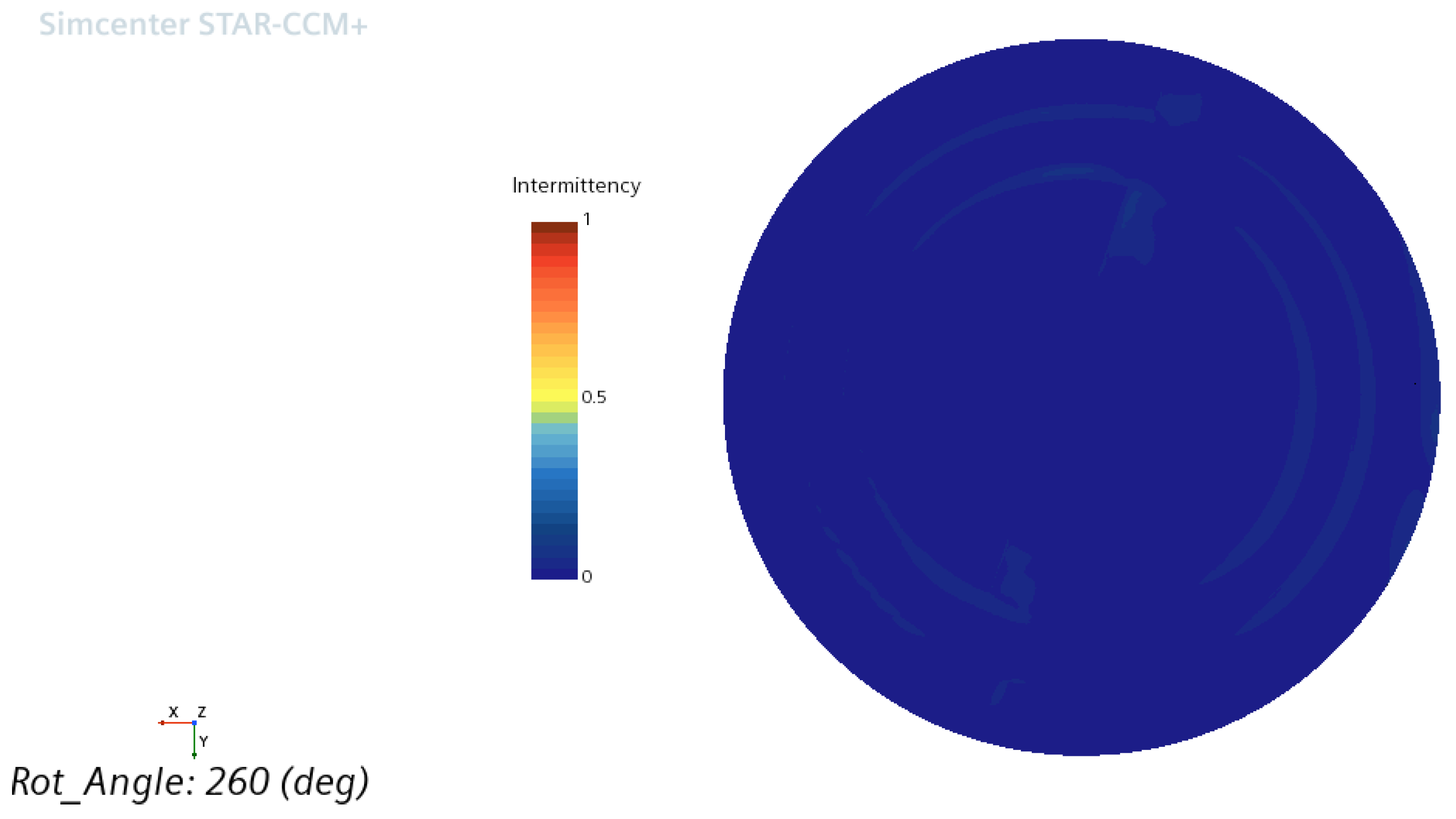
Moreover, the concept of intermittency associated with the gamma transition model was exploited to predict the onset of flow transition within the gap. In detail, the intermittency assumes a unit value when a fully turbulent flow is entered, while a fully laminar flow is predicted in which the intermittency becomes zero. In Figure 16, a section view of the clearance region at any slipper’s angular position displays a diffused null intermittency, thus remarking on the laminar nature of the flow. For the sake of completeness, a qualitative description of the pressure distribution within the three-dimensional fluid domain at the same instant of time is depicted in Figure 17.

4. Discussion and Conclusions

This manuscript presented a CFD methodology for the analysis of the dynamic slipper–swash plate interface in axial piston pumps and motors under actual operating conditions, and an industrial slipper design was considered as test case. The DFBI morphing technique was used to instantly update the position of the slipper, as well as to predict the hydrostatic and hydrodynamic forces acting on the real component. The repulsive force produced by the slipper–swash plate collision was further monitored, and a new coefficient was introduced to estimate the metal contact between parts as a function of the axial forces acting on the component. In detail, a sinusoidal curve for B_G was observed with a decreasing trend along the suction interval and a corresponding increment during supply. At each stage, this result was further suggested by constant hydraulic lift opposing the variable piston force pushing the slipper against the swash plate. The largest discrepancy between the external thrust force and the hydraulic lift on the slipper was measured at the high-pressure transition, in which the maximum piston force was transmitted to the slipper through the ball joint. At this point, a global minimum value of B_G, i.e., 0.62, was measured, indicating the highest slipper instability. Moreover, the primary correlation between the leakage flow and the working pressure was pointed out, with a secondary effect produced by the flow area or, in other terms, the clearance height. A non-uniform pressure distribution was observed through the gap due to the tilted position of the slipper during actual pump-operating conditions, but no significant effects were registered on the hydraulic lift because of the short distance between the grooves, which resulted in a concentrated pressure drop. Therefore, the serious possibility of neglecting secondary hydrodynamic effects induced by slipper tilting in the design stages of vented grooved slippers was outlined in this paper. Furthermore, the laminar behavior of the flow inside the gap was confirmed by a null intermittency along an entire revolution of the pump shaft. In conclusion, despite having known limitations related to the impossibility of simulating an effective zero gap between colliding surfaces, the proposed numerical approach represents an extremely advanced and powerful tool for the slippers’ design in axial piston machines. More works are expected in the future to further investigate the effects of different pump-operating conditions, e.g., high working pressure and variable displacement operations, and different slipper designs.