Intelligent Unsupervised Network Traffic Classification Method Using Adversarial Training and Deep Clustering for Secure Internet of Things ^†

Abstract

Network traffic classification (NTC) has attracted great attention in many applications such as secure communications, intrusion detection systems. The existing NTC methods based on supervised learning rely on sufficient labeled datasets in the training phase, but for most traffic datasets, it is difficult to obtain label information in practical applications. Although unsupervised learning does not rely on labels, its classification accuracy is not high, and the number of data classes is difficult to determine. This paper proposes an unsupervised NTC method based on adversarial training and deep clustering with improved network traffic classification (NTC) and lower computational complexity in comparison with the traditional clustering algorithms. Here, the training process does not require data labels, which greatly reduce the computational complexity of the network traffic classification through pretraining. In the pretraining stage, an autoencoder (AE) is used to reduce the dimension of features and reduce the complexity of the initial high-dimensional network traffic data features. Moreover, we employ the adversarial training model and a deep clustering structure to further optimize the extracted features. The experimental results show that our proposed method has robust performance, with a multiclassification accuracy of 92.2%, which is suitable for classification with a large number of unlabeled data in actual application scenarios. This paper only focuses on breakthroughs in the algorithm stage, and future work can be focused on the deployment and adaptation in practical environments.

1. Introduction

The continuous development and popularity of the Internet of things (IoT) has enabled different sectors of the economy to combine traditional business models with the Internet, creating new solutions, e.g., smart transportation, environmental protection, e-government, safe home, industrial monitoring, etc., [1,2]. However, a large number of interconnected devices leads to poor synchronization protection and management challenges, which may affect the overall security and reliability of the network. Therefore, to provide better services for network users and improve the effectiveness of network management, an efficient network traffic classification (NTC) and supervision is necessary. In NTC, the network packets are captured to determine their identity. The effective NTC can guarantee the quality of network service and intrusion detection system (IDS) [3,4,5].

In the era of big data, NTC has to handle a large quantity of network traffic data, which leads to a high computational complexity and slow classification time [6]. Early NTC methods used Transmission Control Protocol (TCP) or User Datagram Protocol (UDP) ports to distinguish between different network traffic [7]. These methods are simple to use and have a high classification efficiency. However, with the continuous development of the Internet, there are many applications in the network environment that do not follow the established port label or directly hide the ports used by applications. This led to the gradual elimination of port-based traffic classification methods and the rise of deep packet inspection (DPI)-based classification technology. DPI-based technologies are not restricted by network ports and use the unique identifiers in the application layer directly to classify traffic [8]. However, because the use of application-layer data may violate user privacy, and the method cannot recognize encrypted data, DPI-based classification technology has gradually faded out of the NTC field. To address these challenges, researchers have introduced feature selection techniques [9]. Feature selection is the process of selecting the most effective subset of features that compose the entire dataset, and a good subset of features is one that contains features that are highly related to but not related to each other. These features are also the most common reason why network classification systems use feature selection technology. Collected network traffic data usually include information such as source IP, destination IP, source port, destination port, and number of bytes, which are used to distinguish different types of network traffic. Classifying network traffic based on these features technically compensates for the basic technical deficiencies of traditional port-based and DPI-based detection. At the same time, these features do not contain valid information on the message, thus avoiding the disclosure of user privacy. However, there are many features of network traffic, and the number of available features identified in current academic research has reached 240 [10]. For some network traffic, it is too redundant to use all features for classification, which will not only increase the complexity of the classification model, but also reduce the classification accuracy.

In this paper, we propose an adversarial autoencoder (CAAE) network to extract the most relevant features of complex network traffic. The combination of adversarial training and autoencoder can greatly reduce the feature dimension of the original network traffic, and at the same time, filter out the most effective feature information. The basic idea of adversarial training is to continuously generate and learn adversarial samples during network training. For example, according to the minimax formula, adversarial samples are searched for by maximizing the loss function in the inner layer, and then adversarial samples are learned in the outer layer to minimize the loss function. The neural network obtained through adversarial training has more adversarial robustness compared to ordinary autoencoders. The collected network traffic samples usually do not contain category information, so this paper uses an unsupervised clustering model to study. To avoid the mismatch between the selected features and the clustering model, we propose an optimization method, DC-CAAE, based on the CAAE feature extraction. Deep clustering (DC) enables the low-dimensional features to retain the original data structure and information, while making the differences between different data more obvious, thus achieving better clustering results [11]. The main contributions of this paper are as follows:

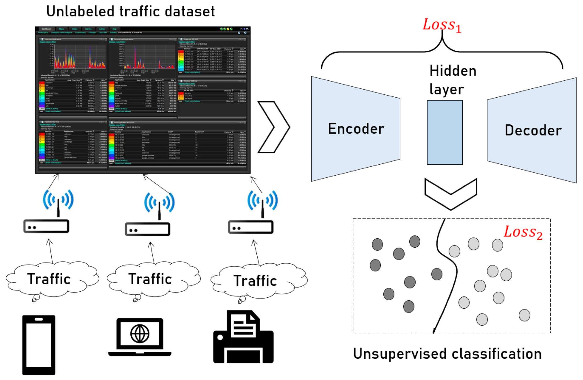
• We propose a new unsupervised NTC method based on adversarial training and deep clustering, where deep clustering can learn more features on the basis of pretraining, and maintain the stability of the detector.
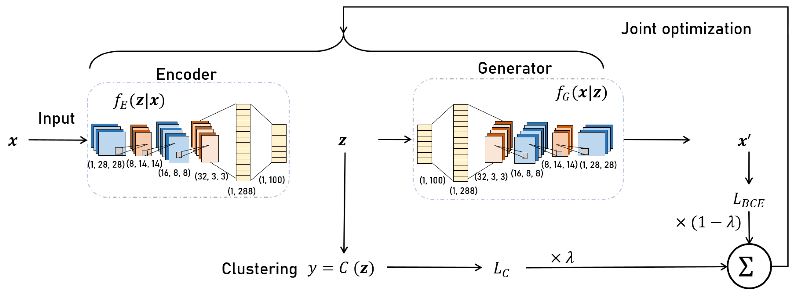
• To avoid a cluster collapse due to deep clustering, we apply a combination of cluster loss and adversarial training loss instead of a single cross-entropy loss. At the same time, CAAE is introduced to reduce the dimension of the feature, which avoids the high complexity of the deep learning model caused by the high-dimensional original network traffic features.
• We evaluate the proposed method on network traffic datasets collected in the real environment. The experimental results show that this method has a good clustering effect, and the multiclassification accuracy reaches 92.2%, which is suitable for industrial scenes with a large number of unlabeled data samples.

2. Related Work

2.1. Traditional NTC Methods

In the early days of NTC development, to solve the problem of traffic classification, different TCP or UDP protocol ports were used to determine the type of traffic, such as those specified by the Internet Assigned Numbers Authority (IAIA) [12] or those widely used by the conventions [13]. However, today more and more traffic cannot be classified by this scheme. In practical applications, the network ports of servers do not always use the ports nominally associated with their applications, and such behavior is not always malicious. For example, users running Web or file transfer protocol (FTP) servers on alternate ports lack administrator privileges. Users running servers that provide nonweb applications on port 80/TCP bypass the firewall of the system to avoid security and policy implementation monitoring [14]. A. Madhukar et al. [15] compared three methods to classify peer-to-peer (P2P) applications: port-based classification, application layer signature, and transport layer analysis. Their experiments showed that nearly 70% of Internet traffic could not be identified simply by port-based methods. DPI technology mainly analyzes the payload of data packets in the network traffic. If the payload part can match with the known application program or protocol in some characters, then the network flow can be roughly considered as the known application program or protocol. The ML-based method uses an ML algorithm to classify network traffic [16]. Byte sequences and statistical features of packets or flows in traffic data are the most common features used by ML-based network flow classifiers. ML-based methods rely on statistical methods to extract features from datasets, but network traffic data are usually large, and statistical extraction methods are often prone to lose important information.

2.2. DL-Based NTC Methods

Deep learning has made great progress on complex problems in computer vision and natural language processing, which also makes more people begin to use deep learning methods to study network traffic in the field of network security [17]. Deep learning can directly learn useful features from the original traffic data, which, to a certain extent, solves the problem of the high cost of artificial feature extraction [18]. R. Zhao et al. [19] proposed a traffic recognition method for the Internet of things based on a lightweight deep neural network, which realized an effective feature extraction at a low cost. The extended compression structure, antiresidual structure, and channel shuffle operation were used to optimize the classifier to solve the problem of uneven sample distribution. The above SL-based methods usually need to include a large number of labeled datasets for training. However, the data obtained in practical applications do not have label information, and the workload of labeling the data is large, so it is difficult to apply them to NTC practice. J. Ning et al. [20] proposed a malware classification method based on semi-supervised learning to reduce the dependence of the classification model on labeled data. Integrated transfer learning and domain adaptive greatly improved the classification accuracy.

In order to get rid of the dependence on data labels and increase the generalization of the model, the method based on unsupervised learning has a good application market. In order to learn features more suitable for unsupervised classification tasks from the original data, P. Huang et al. [21] imposed a position-preserving constraint on the feature representation it learned from the original data to better suit the unsupervised classification task in order to embed the original data into their underlying manifold space. Finally, k-means was used for clustering, and good performance was obtained. P. Li et al. [22] proposed an improved stacked AE, which could learn complex relationships on multisource network flows by stacking several basic Bayesian autoencoders. However, the overlap of multilayer autoencoders increased the computation time. Both of the above unsupervised methods optimize the classification model for feature selection, and the performance of the clustering algorithm cannot be optimized. To address these challenges, S. Shah et al. [23] proposed an algorithm that combined a nonlinear dimension reduction with clustering methods. The compressed low-dimensional data of the deep neural network were fed into the cluster model for retraining. This method combined a dimension reduction with clustering as a global optimization objective, avoiding cluster mismatch caused by no clustering training. The deep clustering method improved the accuracy of the clustering. In conclusion, the deep-learning-based NTC method plays an important role in the complex network traffic environment, and improving the accuracy of unsupervised network traffic classification is one of the key points at present. We believe that unsupervised NTC methods for the Internet of things should follow the following principles:

• Robust classification performance: In a real network scenario, any undetected attack may cause the network to crash, resulting in huge losses. Hence, the main goal of NTC method is to continue to accurately classify ordinary traffic and malicious attacks in normal network scenarios.
• Strong model generalization ability: IoT devices are subject to fast-changing attacks, a large number of attacks, and attacks that are good at disguising. Hence, it is necessary to detect with a model that is well adapted to attacks of unknown categories.
• Low model complexity: Network traffic has a large quantity of sample data; hence, it is necessary to use a simple classification model to reduce the detection cost.

Based on the above principles, we studied an efficient unsupervised network traffic classification method, focusing on improving the effectiveness of the feature selection and the accuracy of the deep clustering.

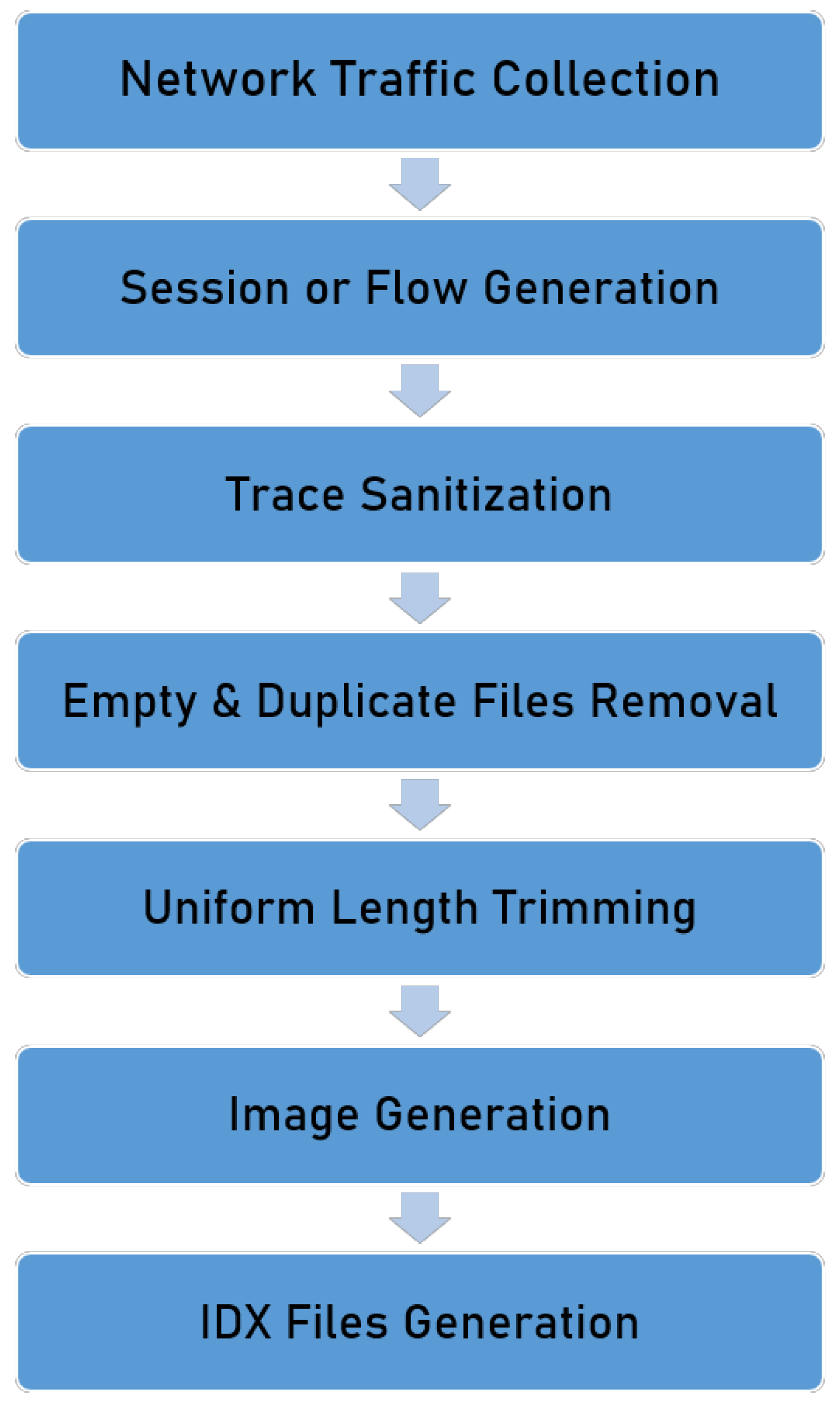
3. Problem Formulation and Dataset Generation

3.1. Problem Description

In unsupervised learning, the label of the sample is unknown, that is, the dependent variable is not as clearly labeled as in supervised learning, such as number size, animal species, or flower category. Therefore, in practical applications, unsupervised learning has a large application market. The types of network traffic attacks become more and more varied with the beginning of the era of the Internet of Everything (IoE), and unknown attack types endlessly emerge. Therefore, it is an inevitable trend to optimize the network traffic classification system using unsupervised networks. In unsupervised learning, when the output of the system is finite and discrete, the prediction of the system can be regarded as a classification problem. The classification model or classification decision function learned from the original data is called a classifier, and the process of classifying from input to output is called classification. The output results become classes. When the number of classes is greater than one, it is called a multiclassification problem. This paper mainly discusses the multiclassification problem.

In unsupervised learning, the problem we have to deal with is to train a reliable unlabeled feature extractor. There are two main ways to do this. One is to optimize the loss function of pseudolabels according to the principle of reducing the distance within clusters and expanding the distance between clusters. The second is to use additional tasks to help train the feature extractor. For clustering methods with special feature extractors, such as autoencoders, the loss of reconstruction can be interpreted as an additional task, as shown in Figure 1.

The process of training reconstruction loss is also a process of data feature dimensionality reduction. The so-called dimension reduction in machine learning refers to the mapping of data points from the original high-dimensional space to a low-dimensional space using some mapping method. The feature dimension has a great influence on the computational complexity of classifier. The computational complexity increases exponentially with the number of neurons and the number of layers of the neural network [24]. The essence of dimension reduction is to learn a mapping function $f:\mathit{x}\to \mathit{z}$, where $\mathit{x}$ is the representation of the original data points, and at present, most methods use a vector representation. $\mathit{z}$ is a low-dimensional vector representation of the mapped data points, and $\mathit{z}$ is usually smaller than $\mathit{x}$ (although increasing the dimension is also possible). f may be explicit or implicit, linear or nonlinear. Data in the NTC field are often characterized by a large number of features, a large quantity of data, and complex features. The performance of traditional linear dimensionality reduction methods such as principal component analysis (PCA) and linear discriminant analysis (LDA) is poor when extracting complex feature tasks. Therefore, a nonlinear feature dimensionality reduction method is more suitable for network traffic classification. The autoencoder feature dimensionality reduction method is discussed as an example below.

An autoencoder is the process of encoding the original data, reducing the dimensions, and discovering the rules between the data. The whole autoencoder can be described as:

$$f_{Decoder}\left(f_{Encoder}\left(\mathit{x}\right)\right)={\mathit{x}}^{\prime },$$

(1)

where the output ${\mathit{x}}^{\prime }$ is close to the original input $\mathit{x}$. The purpose of the network is to reconstruct its input so that its hidden layer can learn the good representation of the input. If the input is exactly equal to the output, i.e., $f_{Decoder}\left(f_{Encoder}\left(\mathit{x}\right)\right)=\mathit{x}$, the network is meaningless. Therefore, some constraints need to be imposed on the self-encoder so that it can only be approximately copied. These constraints force the model to consider which parts of the input data need to be copied first, so it can often learn the useful characteristics of the data. Generally, there are two kinds of constraints [25]: one is to make the hidden dimension smaller than the input dimension, which is called undercomplete; the other is to make the dimension of the hidden layer larger than the dimension of the input data, which is called overcomplete. In a complex network traffic environment, the undercomplete method is generally used to reduce the computational complexity. During the training process, a target loss function is used to measure the similarity between input and output data, which is expressed as follows:

$$Loss1:f_{recon}\left(\mathit{x}\right)={∥\mathit{x}-f_{Decoder}\left(f_{Encoder}\left(\mathit{x}\right)\right)∥}^2,$$

(2)

where $f_{recon}(·)$ is the loss function to measure the difference of input data $\mathit{x}$ and output data ${\mathit{x}}^{\prime }$.

Unsupervised clustering divides datasets into different classes or clusters according to specific criteria, such as a distance. It makes the data samples in the same cluster as similar as possible, and the database samples in different clusters as different as possible. That is, the intraclass distance is the smallest, and the interclass distance is the largest. The specific implementation process of an unsupervised clustering algorithm can be roughly divided into the following four steps:

• Randomly set $\left\{C_1,C_2,\cdots ,C_k\right\}$ initial cluster centers, and k represents the number of clusters.
• For each sample data point $\left\{{\mathit{x}}_1,{\mathit{x}}_2,\cdots ,{\mathit{x}}_n\right\}$, where n is greater than k, each object has attributes of m dimensions. Calculate its distance from the center of each cluster and divide each sample into the nearest cluster.
• Recalculate the average value of each cluster as the new cluster center, and update the original cluster center.
• Repeat the above two or three steps to iterate continuously until the center of each cluster does not change.

Generally speaking, in clustering algorithms, the attributes of samples are mainly represented by their relative distances in the feature space. This makes the concept of distance very important for clustering. The Euclidean distance from each object to each cluster center is calculated as follows:

$$Loss2:dis({\mathit{x}}_i,C_j)=\sqrt{\sum _{t=1}^m{({\mathit{x}}_{it}-C_{jt})}^2}$$

(3)

where t represents the tth attribute of each object. Hence, the focus of this paper is to optimize and adjust the model from the two directions of complex data feature dimension reduction and unsupervised clustering.

3.2. Dataset Introduction

The USTC-TFC2016 dataset [26] contains 10 types of malware traffic and 10 types of benign traffic. It takes the original data as input and classifies the original data by converting it into images. The dataset has a capacity of 3.71 Gb, including 228,762 malware instances (packets) and 309,980 normal instances (packets), all in pcap format. The collected network traffic data contains information such as source IP, source port, target IP, target port and transport level protocol and so on. We process it through four data preprocessing steps, as shown in Figure 2. In this paper, the original dataset was segmented into a training set and a testing set, and the split ratio was set to 3:1. The data classes and sample quantity of the dataset are shown in

Table 1. Data segmentation of the training set and test set.

Benign Data	Training Det	Testing Set	Malicious Data	Training Set	Testing Set
BitTorrent	5049	1716	Cridex	5595	1805
Facetime	4045	1355	Geodo	4543	1490
FTP	4660	1542	Htbot	4346	1384
Gmail	5828	1938	Miuref	3476	1145
MyDQL	4911	1606	Neris	5714	1940
Outlook	5014	1758	Nsis-ay	4100	1362
Skype	4275	1414	Shifu	6451	2220
SMB	4248	1448	Tinba	5772	1882
Weibo	4510	1496	Virus	4399	1473
World of Warcraft	5313	1782	Zeus	4075	1353

.

4. The Proposed DC-CAAE Method

In unsupervised clustering tasks, there are mainly two methods to obtain labels [27]. The first method is to embed data into low dimensional features, and then cluster the embedded features with traditional clustering methods such as k-means algorithm. The second method jointly optimizes the feature extractor and clustering results. We call these two methods separation analysis and joint analysis, respectively. A separation analysis means that learning features and clustering data are executed separately, and low dimensional features are clustered after the dimensionality reduction of data features. To solve the problem that the representation learned by the separation analysis is not oriented toward clustering due to its inherent characteristics, the joint analysis shows its advantages. In this paper, we propose to use a DC method of joint analysis, which imposes the reconstruction error as a constraint on the basis of the clustering error. These two constraints improve the clustering performance, reduce the distance within a cluster and expand the distance between clusters. The proposed model framework is shown in Figure 3. Algorithm 1 summarizes the process of the proposed method. Details of each processing stage of the method are shown below.

Algorithm 1 Pseudocode of the proposed adversarial-training-based DC-CAAE method for NTC.

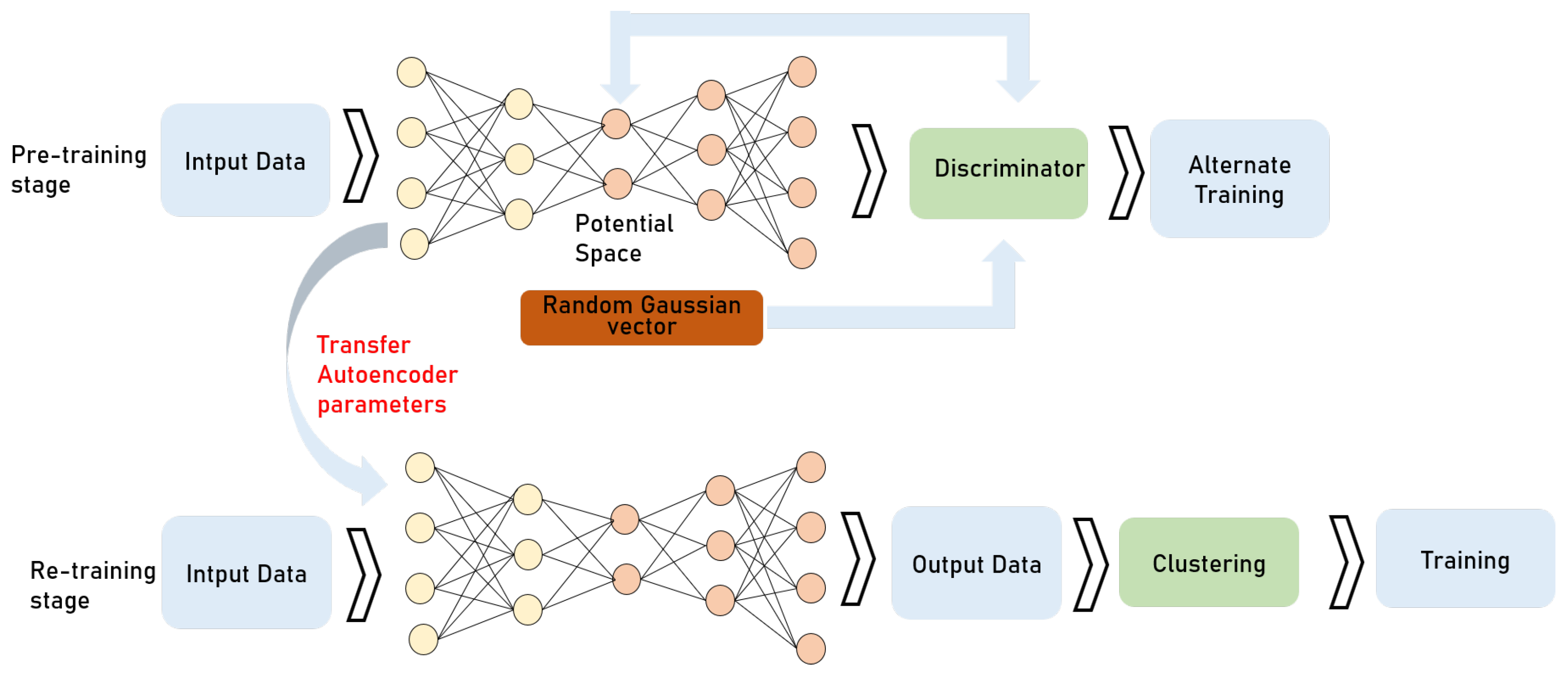
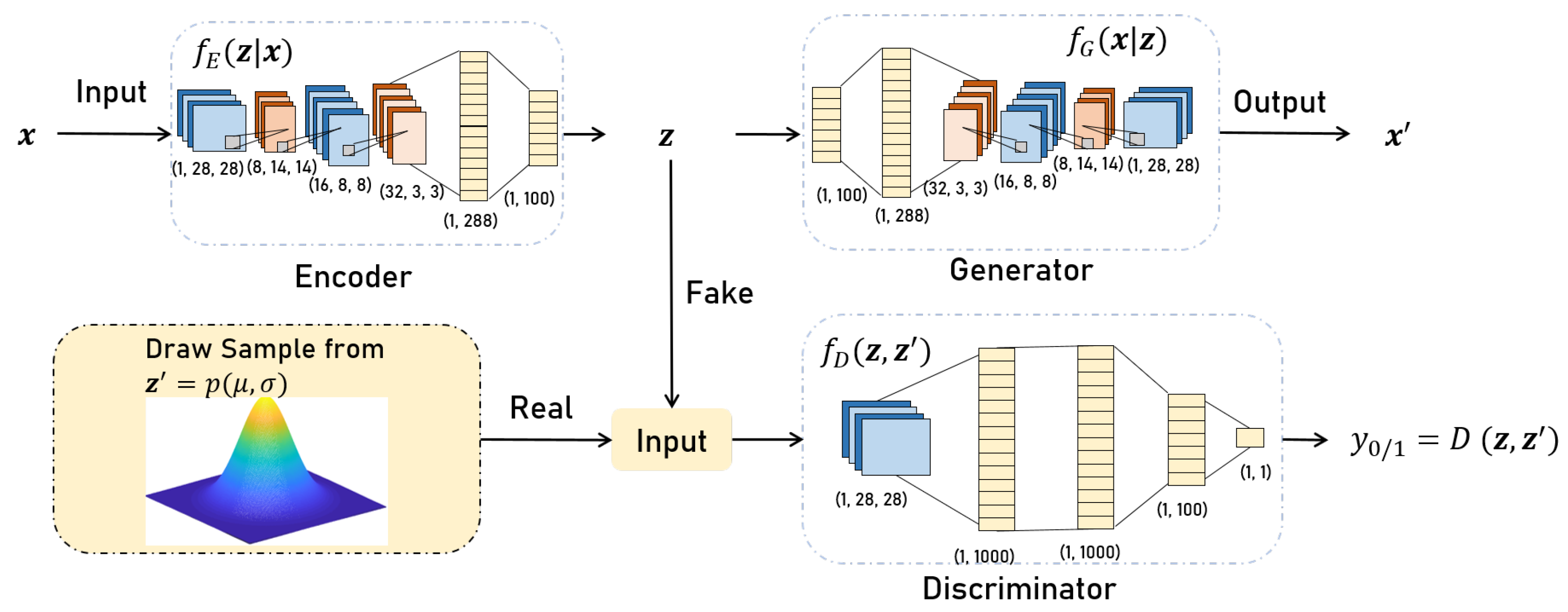
Require:  Samples X; reconstruction samples $X^{{}^{\prime }}$; potential representation Z; random Gaussian distribution G; pretraining hyperparameters ${\theta }_{pre}$; retraining hyperparameters ${\theta }_{re}$; maximum epochs of AAE $E_{CAAE}$; maximum epochs of DC $E_{DC}$; hyperparameter $\lambda$; the number of batches in a training iteration B. Ensure:  Clustering results C. 1: [Pretraining stage]: for $i=1,2,\cdots ,E_{CAAE}$ do:    for $t=1,2,\cdots ,B$ do: Sample a batch dataset $X_b$    [Forward propagation]:       $Z_{pre},X_{pre}^{{}^{\prime }}\leftarrow Ne{t}_{CAAE}(X_b,G)$       $Loss1\leftarrow L_{BCE}(X_b,X_{pre}^{{}^{\prime }})$       $Loss2\leftarrow L_D(Z_{pre},G)$ [Backward propagation]:       Alternately minimize $Loss1,Loss2$       Update ${\theta }_{pre}$ with $Loss1,Loss2$ 2:    end for 3: end for 4: Save ${\theta }_{pre}$. 5: [Deep clustering stage]: 6: Randomly initialize the parameters ${\theta }_{re}$ 7: Load ${\theta }_{pre}$ for $i=1,2,\cdots ,E_{DC}$ do:    for $t=1,2,\cdots ,B$ do: [Forward propagation]:       $Z_{re},X_{re}^{{}^{\prime }}\leftarrow Ne{t}_{CAE}\left(X\right)$       $C\leftarrow Ne{t}_{DC}\left(Z_{re}\right)$       $Loss\leftarrow (1-\lambda )L_{BCE}(X,X_{re}^{{}^{\prime }})+\lambda L_C(X,C)$ [Backward propagation]:    Update ${\theta }_{re}$ with $Loss$ 8:    end for 9: end for 10: Save ${\theta }_{re}$. 11: Test and save the performance of the DC-CAAE model 12: Return DC-CAAE model

4.1. CAAE Structure

A CAAE network combines a CAE with adversarial training, and its core is still to use a generator G and a discriminator D for adversarial learning to distinguish between real data and fake data. However, unlike an ordinary adversarial training network, the data that CAAE needs to distinguish are not a natural image but a coded vector $\mathit{z}$. The real data and fake data to be identified are generated by the encoder in the CAE and a predefined random probability distribution, respectively. Finally, the network used for image generation is not the former generator, but the decoder in the CAE. Its model architecture is shown in Figure 4.

The $\mathit{x}$ in the CAAE represents the image data of the preprocessed network traffic. Enter $\mathit{x}$ into a CAE and have the encoder encode it to generate a potential vector $\mathit{z}$. The decoder then attempts to decode the potential vector and regenerate the image data ${\mathit{x}}^{\prime }$. The key to this model is that the encoder and the discriminator form an adversarial network. The discriminator predicts whether $\mathit{z}$ comes from real or fake data by learning constantly. The whole process of adversarial learning can be thought of as constantly adjusting the encoder to bring the resulting data distribution closer to a predefined $p\left({\mathit{z}}^{\prime }\right)$.

4.2. The Basic Principles of the CAAE

Set network traffic $\mathit{x}$ as the real picture data after processing, that is, the input of the CAAE model is multiple network traffic vectors. We can map network traffic $\mathit{x}$ to the feature vector based on encoder E, that is, $E\left(\mathit{x}\right)=\mathit{z}$, where the dimension of the network traffic features is 100. The CAAE is a neural network that learns valid features in an unsupervised learning method. The reconfiguration of generator G forces the encoder to learn basic potential features, that is, ${\mathit{x}}^{\prime }=G\left(\mathit{z}\right)$. The core appeal of our method is to always maintain the extracted features to convey the characteristics of the original data as much as possible. Therefore, in this process we want ${\mathit{x}}^{\prime }$ to be as similar as possible to $\mathit{x}$, which can be expressed by minimizing the loss function:

$$L_{BCE}=-({\mathit{x}}^{\prime }log\mathit{x}+(1-{\mathit{x}}^{\prime })log(1-\mathit{x})),$$

(4)

At the same time, $\mathit{z}$ is constrained by a random Gaussian distribution. Assume that $p(\mu ,\sigma )$ is an a priori distribution and ${\mathit{z}}^{\prime }\sim p(\mu ,\sigma )$ is used to describe a random Gaussian process base on $p(\mu ,\sigma )$, where $\mu$ is the mean and $\sigma$ is the variance. When the distribution of the training data is expressed as $p_{data}\left(\mathit{x}\right)$, the specific training implementation on the encoder and discriminator can be achieved through the maximum-minimum objective function:

$$\begin{array}{cc}\hfill \underset{E}{min}\underset{D}{max}V(D,E)& =E_{{\mathit{z}}^{{}^{\prime }}\sim p(\mu ,\sigma )}(lnD\left({\mathit{z}}^{{}^{\prime }}\right))\hfill \\ \hfill & +E_{z\sim p_{data}\left(\mathit{x}\right)}(ln(1-D(E\left(\mathit{x}\right)\left)\right)),\hfill \end{array}$$

(5)

where $D(·)$ is the output function of the discriminant model, the output is a real value ranging from 0 to 1, which is used to judge whether the data are false or not. The expression $E_{{\mathit{z}}^{{}^{\prime }}\sim p(\mu ,\sigma )}(lnD\left({\mathit{z}}^{{}^{\prime }}\right))$ is to make the real data put into the calculated value output by the discriminant model $D(·)$ and the whole formula subvalue as large as possible. The expression $E_{z\sim p_{data}\left(\mathit{x}\right)}(ln(1-D(E\left(\mathit{x}\right)\left)\right))$ is to make the calculated value of the false data from the output of the discriminant model $D(·)$ as small as possible and the whole formula as large as possible. This integration is to make the objective function as large as possible, so the gradient can be improved according to the objective function during training.

4.3. CAAE Training Process

Before the training starts, we divide the dataset into two parts, the training set and the test set. The training set is used to train the CAAE network, and the test set is used to verify the effectiveness of the training. The basic network architecture of the encoder, generator and discriminator in the CAAE is shown in

Table 2. Details of the CAAE model.

Layer	Encoder	Generator	Discriminator
Input	Input	Input	Input
Layer 1	Conv2d (1, 8, 3, 2, 1)	Linear (100, 1000)	Linear (100, 1000)
Layer 2	Conv2d (8, 16, 3, 2, 1)	Linear (1000, 288)	Linear (1000, 1000)
Layer 3	Conv2d (16, 32, 3, 2, 0)	ConvTranspose2d (32, 16, 3, 2, 0)	Linear (1000, 1)
Layer 4	Linear (288, 1000)	ConvTranspose2d (16, 8, 3, 2, 1)	None
Layer 5	Linear (1000, 100)	ConvTranspose2d (8, 1, 3, 2, 1)	None
Output	Output	Output	Output

.

In each batch of the training process, we alternately optimizes (4) and (5), constantly forcing the resulting potential features to more effectively represent key information about network traffic.

4.4. Deep Clustering Structure

In this experiment, we analyzed the methods to improve unsupervised clustering performance from the two perspectives of cluster-loss-oriented and feature-oriented performance. Cluster-loss-oriented performance shows whether there is a loss function that explicitly reduces or widens the distance between clusters. The resulting feature extractor is unreliable during the CAAE training. Therefore, the DC-CAAE-based deep clustering method was optimized using the traditional cluster loss’s extra constraint feature extractor. The basic framework of deep clustering is shown in Figure 5.

4.5. The Basic Principles of Deep Clustering

The hidden features extracted from the CAAE model represent good key features for expressing network traffic data. To further optimize the encoder parameters, we propose a new optimization goal using the joint analysis method. For k-means clustering, the core idea is to make the points within the cluster as close to the center point C as possible. Its clustering objectives can be expressed as:

$$L_C=\sum _{i=1}^n{∥E\left({\mathit{x}}_{\mathit{i}}\right)-C_i∥}^2,$$

(6)

where i represents the cluster category. To ensure the fairness of the experiment in this paper, the clustering method uniformly used the k-means clustering method based on the Euclidean distance. The loss function of the whole DC model consists of the error of the autoencoder in the CAAE and the error of the k-means clustering. The joint loss function is:

$$\begin{array}{cc}\hfill L_{joint}=& (1-\lambda )L_{BCE}+\lambda L_C\hfill \\ \hfill =& (1-\lambda )\left(-({\mathit{x}}^{\prime }log\mathit{x}+(1-{\mathit{x}}^{\prime })log(1-\mathit{x}))\right)\hfill \\ \hfill +& \lambda \left(\sum _{i=1}^n{∥E\left({\mathit{x}}_{\mathit{i}}\right)-C_i∥}^2\right),\hfill \\ \hfill & \mathrm{s}.\mathrm{t}.\lambda \in [0,1]\hfill \end{array}$$

(7)

when $\lambda =1$, the DC model does not calculate the autoencoder loss, it only uses the cluster loss to adjust the neural network parameters. When $\lambda =0$, the DC model does not calculate the cluster loss, but only uses the autoencoder loss to optimize the network parameters. When $0<\lambda <1$, the deep clustering uses both the autoencoder loss and cluster loss to constrain the convolution neural network parameters, which ensures the similarity between the input and output layers of the autoencoder while keeping the clustering’s resulting clusters relatively close.

4.6. Deep Clustering Training Process

The DC contains two modules, CAE and clustering. During training, the losses of the two modules are optimized together via Equation (7). In the backpropagation, the loss $L_{joint}$ is fed back to the encoder to optimize the encoder’s network parameters. After deep clustering, the features extracted by the coding layer are spatially friendly to clustering. This process uses the Adam optimizer, and the learning rate was set to 0.0001. The maximum epoch during DC training was set to 30. The autoencoder network parameters are then loaded from the previous training step into the neural network for deep clustering. The intermediate output $\mathit{z}$ and the sample reconstruction result ${\mathit{x}}^{\prime }$ are calculated by a forward-propagation to obtain the reconstruction error $L_{BCE}$. Then, the cluster calculation is performed. It consists in selecting k initial cluster centers, calculating the distance d between each element in the dataset and each cluster center, obtaining the cluster loss $L_C$, and dividing the samples into the nearest categories. The deep clustering error $L_{joint}$ is computed jointly, and the network parameters are corrected by backpropagation until the loss function converges.

4.7. The Benchmark Methods

4.7.1. PCA-Based Methods

PCA [28] is a common data dimension reduction method, which compresses high-dimensional data by extracting the main feature vectors. PCA maps n-dimensional features to k-dimensions, where $n>k$, where k-dimensional features become the principal components. In the early research stage of network traffic classification system, PCA was widely used as a convenient and efficient dimension reduction algorithm. In this paper, to ensure the fairness of the comparative experiment, the dimensions of the original data were reduced to 100.

4.7.2. CAE/CVAE-Based Methods

The CAE network was originally designed for unsupervised representation of data. It can learn a nonlinear function mapping. The use of depth CAE [29] allows the feature extractor to learn the features one wants to cluster. CAE compresses the data to low dimensions, and then reconstructs the input to find the representation of low-dimensional data. CVAE [30] is a variant of CAE. CVAE can solve the problem that CAE cannot generate arbitrary data. It can directly generate a hidden vector z through the model, and the generated $\mathit{z}$ contains both data information and noise, so using different $\mathit{z}$’s can generate endless new data. The dimensions of the original data were reduced to 100.

4.7.3. DC-Based Methods

Due to the low efficiency of the similarity measurement methods used, the performance of traditional clustering methods on high-dimensional data is poor, and the computational complexity on large-scale datasets is high. The dimensionality reduction and clustering of high-dimensional data are often two separate parts, and such a structure can lead to mismatches between the dimensionality reduced data features and the clustering method, never reducing the accuracy of clustering. The research shows [31] that the performance of a feature extractor can be greatly improved by jointly optimizing the data dimension reduction and clustering tasks. This method is based on the premise that the sample data are obtained through a potential feature transformation, called deep clustering [32]. Deep clustering connects data dimensionality reduction and clustering through deep learning, and the joint training enables the clustering and feature extraction to be carried out within a unified framework.

5. Simulation Results and Discussions

5.1. Simulation Setup and Evaluation Metrics

5.1.1. Simulation Setup

The server used in this experiment was a Geforce RTX 2080 Ti GPU with 11G of RAM, the programming language was Python, and the programming framework was Pytorch. The experimental results were evaluated using Scikit-learn 1.0.2. The dataset used in the experiment was USTC-TFC2016 [26], with about 120,000 training samples. Detailed simulation parameters are shown in

Table 3. Simulation environment and parameters.

Parameter	Value
Dataset	USTC-TFC2016
Input data dimension	(28, 28, 1)
Hidden feature dimension	100
Environment	Python 3.10.4, Scikit-learn 1.1.0,  Torch 1.11.0, Numpy 1.22.3
Device	GeForce RTX 2080 Ti
Pretraining hyperparameters	Optimizer	Adam
	Weight_decay	0
	Batch size	128
	Learning rate	0.00001
	Epoch	80
Deep clustering hyperparameters	Optimizer	Adam
	Weight_decay	0
	Batch size	128
	Learning rate	0.0001
	Epoch	30

.

5.1.2. Evaluation Metrics

The evaluation metrics of machine learning methods vary in different research fields. This paper studied the unsupervised network traffic clustering problem, so the evaluation metrics used were also based on the clustering model. The cluster validity evaluation metrics used in this paper were composed of the internal validity metric silhouette coefficient and the external validity evaluation metrics normalized mutual information (NMI), adjusted Rand index (ARI), clustering accuracy (AC), and v-measure, respectively. When evaluating the classification model, the most common metric is the classification accuracy. Unsupervised learning’s training process does not involve sample labels, so the accuracy calculation method is different from that of supervised learning. Assuming there are N samples, the label produced by the ith sample cluster is $p_i$, and the true label is $y_i$, the formula for calculating the accuracy is:

$$AC=\frac{1}{N}\sum _{i=1}^N\delta (y_i,\mathrm{map}\left(p_i\right)),$$

(8)

where map$(·)$ represents the redistribution of clustering labels, which is generally achieved by the Hungarian algorithm [33]. $\delta (·)$ stands for indicating function

$$\delta (x,y)=\left\{\begin{array}{cc}1& \mathrm{if}x=y\\ 0& \mathrm{otherwise}\end{array}\right..$$

(9)

NMI is often used to measure the degree of agreement between two clustering ${\pi }_K$ and ${\pi }_L$ results, and it can be expressed as

$$NMI({\pi }_K,{\pi }_L)=\frac{{\sum }_{k=1}^K{\sum }_{l=1}^L{n}_l^{k}log\left(\frac{n{n}_l^k}{n^k{n}^l}\right)}{\sqrt{({\sum }_{k=1}^K{n}^{k}log\left(\frac{n^k}{n}\right))({\sum }_{l=1}^L{n}^{l}log\left(\frac{n^l}{n}\right))}},$$

(10)

where $n^k$ is the kth cluster generated by the cluster, and $n^l$ is the number of data samples from the lth cluster in the real cluster. $n_k^l$ is the number of data samples shared by the kth cluster result and the lth real cluster. ARI is a real value that reflects the degree of overlap between the cluster and the actual cluster. The larger the value, the better the clustering effect. Its mathematical expression is given by

$$ARI=\frac{RI-E\left(RI\right)}{max\left(RI\right)-E\left(RI\right)},$$

(11)

$$RI=\frac{a+d}{a+b+c+d},$$

(12)

where a denotes the same class of samples clustered in the same cluster, b denotes different classes of samples clustered in the same cluster, c denotes the same class of samples clustered in different clusters, and d denotes different classes of samples clustered in different clusters. Homogeneity refers to cluster classes with the same class of samples within a cluster, and completeness refers to samples of the same class being assigned to the same cluster class. V-measure is the harmonic mean of homogeneity and completeness used to express the proximity of the two categories. Its mathematical expression is given by

$$\begin{array}{cc}\hfill v=& \frac{2\times h\times c}{h+c}\hfill \\ \hfill =& \frac{2\times \left(1-\frac{H(C\mid K)}{H\left(C\right)}\right)\times \left(1-\frac{H(K\mid C)}{H\left(K\right)}\right)}{\left(1-\frac{H(C\mid K)}{H\left(C\right)}\right)+\left(1-\frac{H(K\mid C)}{H\left(K\right)}\right)},\hfill \end{array}$$

(13)

where C and K represent clusters and real classes, respectively, $H(·|·)$ represents conditional entropy. As an internal evaluation metrics of clustering, silhouette coefficient combines cohesion and separation to evaluate the clustering effect. Its definition formula is as follows:

$$s_i=\frac{b_i-a_i}{max(a_i,b_i)},$$

(14)

where $a_i$ represents the average distance between sample $x_i$ and other samples in the same class, and $b_i$ represents the minimum of the average distance between sample $x_i$ and other cluster samples. The average value of $s_i$ for all samples is the clustered silhouette coefficient, that is:

$$SC=\frac{1}{N}\sum _{i=1}^N{s}_i.$$

(15)

5.2. Simulation Results and Analysis

5.2.1. Performance Comparison of Unsupervised NTC Methods

In this section, we first compare the accuracy of our DC-CAAE method with PCA, CAE, CVAE, and the corresponding deep clustering method when the potential spatial feature dimension is 100. Then, we compare the simulation results of DC-CAAE under different clustering methods.

It can be seen from the results in

Table 4. Performance comparison between DC-CAAE and other methods.

Methods	NMI	AC	Silhouette Coefficient	ARI	V-Measure
PCA	0.685	0.494	0.326	0.345	0.685
CAE	0.887	0.824	0.526	0.740	0.887
CVAE	0.888	0.830	0.492	0.758	0.889
CAAE	0.882	0.888	0.408	0.796	0.890
DC-CAE	0.873	0.844	0.518	0.736	0.873
DC-CVAE	0.890	0.857	0.481	0.753	0.891
DC-CAAE (proposed)	0.911	0.922	0.422	0.844	0.917

that the performance of the traditional PCA dimension reduction algorithm on the USTC-TFC2016 dataset is not good, and the accuracy of the clustering is only 49.4%. However, the performance significantly improves after using the deep learning method. The clustering accuracy of CAE is 33.0% higher than that of PCA, and its silhouette coefficient is 20.0% higher. This shows that in complex network traffic datasets, the deep learning method will achieve better results than traditional methods. The combination of the CAAE method and DC proposed in this paper further optimizes the feature extractor. After adding the deep clustering module, the performance of the CAE and CVAE models improves. Of course, the CAAE has the greatest improvement. The clustering accuracy of the DC-CAAE method is 92.2%, which is the highest among all methods in Table 4. At the same time, considering NMI, silhouette coefficients, ARI, and V-measure, the DC-CAAE method proposed in this paper still has good advantages.

According to the results in Table 4, in order to avoid the dependence of the results on clustering methods, we used five different clustering algorithms to analyze the stability of the above feature extractors.

It can be seen from

Table 5. The performance of DC-CAAE with different clustering methods.

Methods	NMI	AC	Silhouette Coefficient	ARI	V-Measure
Minibatch k-means clustering	0.894	0.905	0.418	0.829	0.901
Spectral clustering	0.908	0.908	0.444	0.826	0.915
BIRCH	0.903	0.906	0.427	0.819	0.910
GMM	0.904	0.908	0.428	0.822	0.911
k-Means clustering	0.911	0.922	0.422	0.844	0.917

that the performance of k-means, minibatch k-means, spectral clustering, BIRCH, and GMM clustering algorithms on DC-CAAE was similar. The accuracy of the five clustering algorithms was about 90%, and the error was less than 2%. It can be seen that the DC-CAAE method proposed in this paper was stable on the USTC-TFC2016 dataset, and its performance did not change due to the different clustering methods.

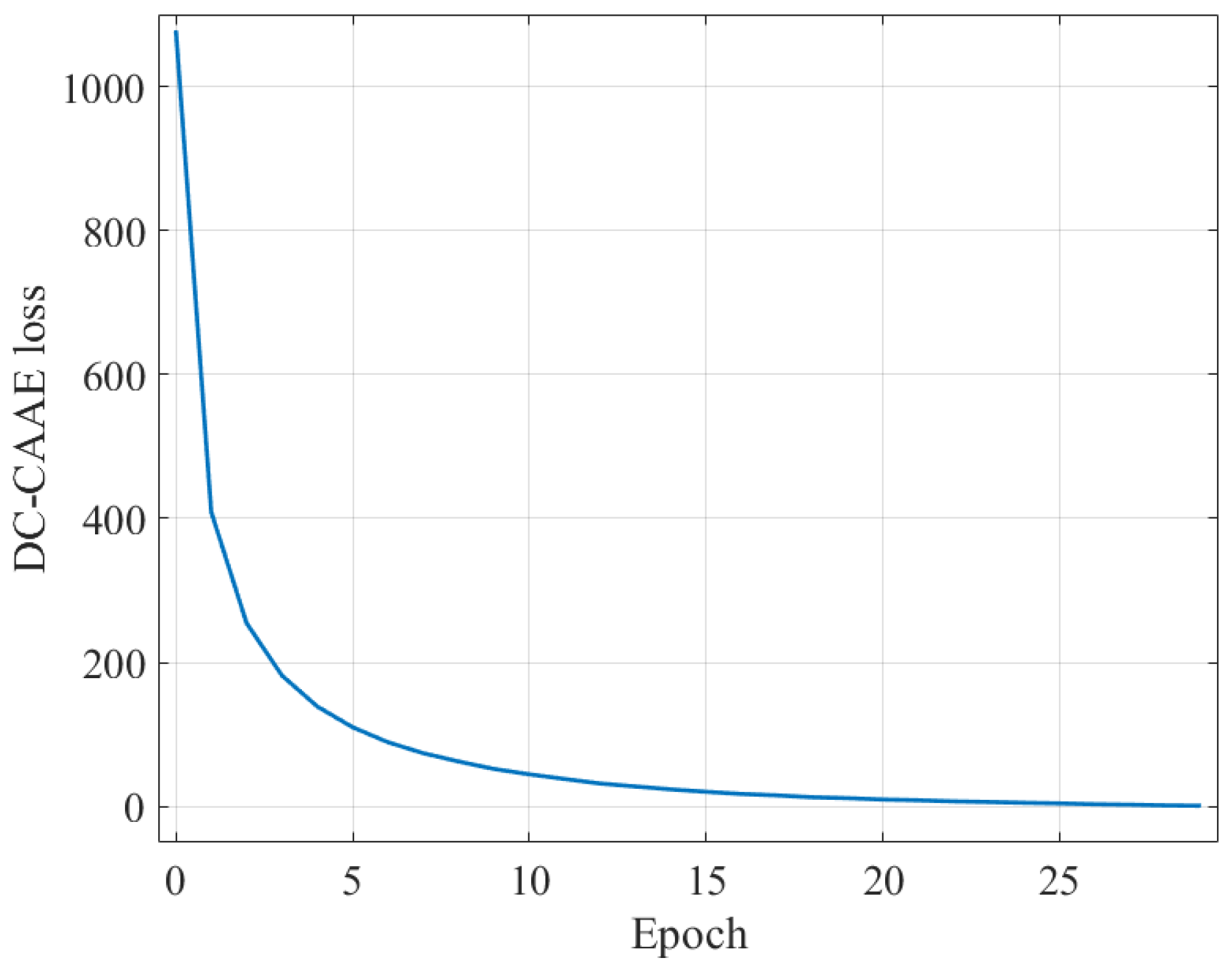
5.2.2. Convergence Analysis

It can be seen from the training process that the loss function of the DC-CAAE method proposed in this paper is a strict convergence process. As shown in Figure 6, the model loss decreases from about 1000 to 1 and tends to be flat after epoch 15. That is to say, the model reaches a stable state after that epoch.

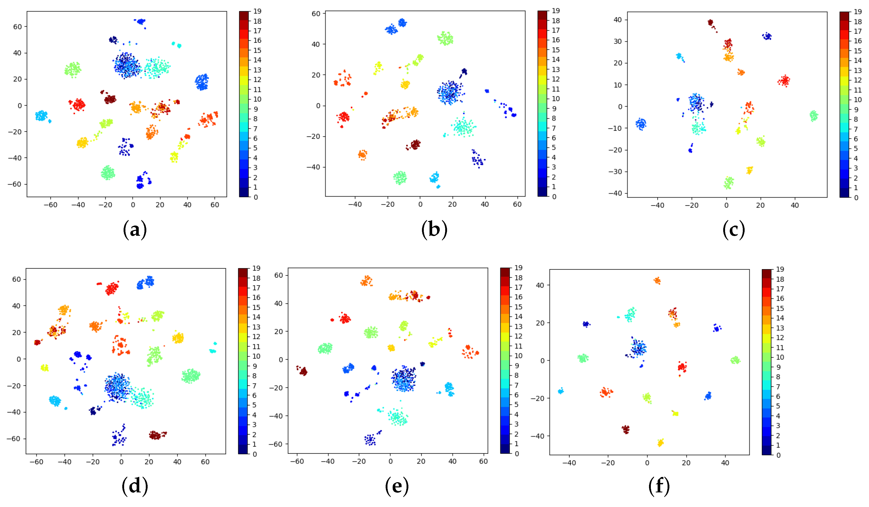
5.2.3. t-SNE Feature Visualizations

In order to more intuitively observe the effect of the DC-CAAE on the data dimensionality reduction, we visualized the output potential representation z and compressed it to a two-dimensional plane for observation. Figure 7 shows the clustering space of different networks, each represented by a different color. All methods reduced the data dimension to 100 dimensions. It can be seen that the distance between each class of features extracted by the ordinary CAE is not obvious, and some classes are mixed together. The DC-CAAE method achieves a more friendly clustering space than the original coded image space and the space before the joint training.

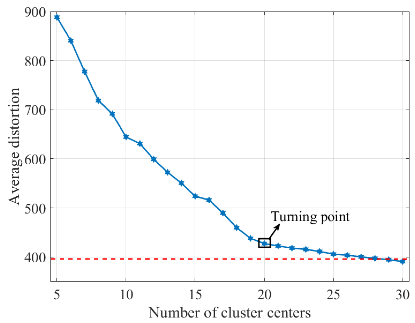
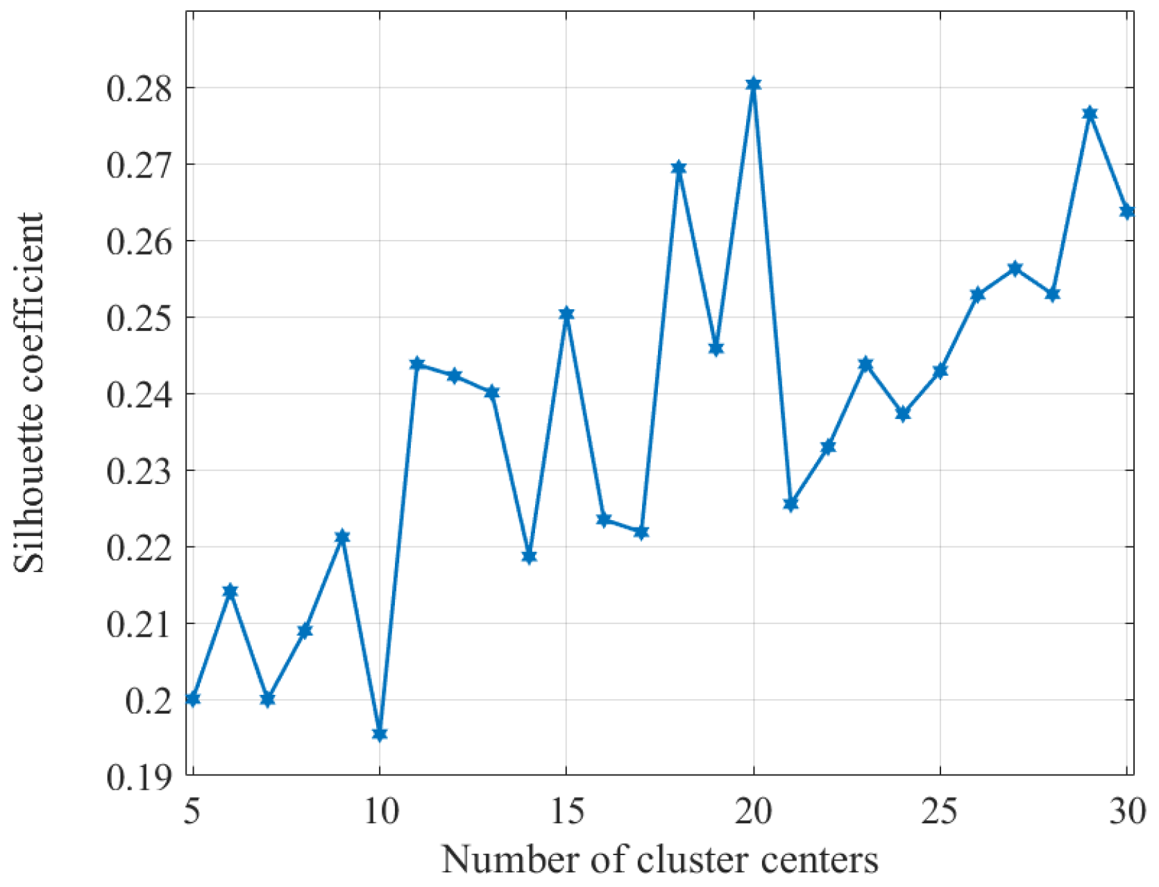
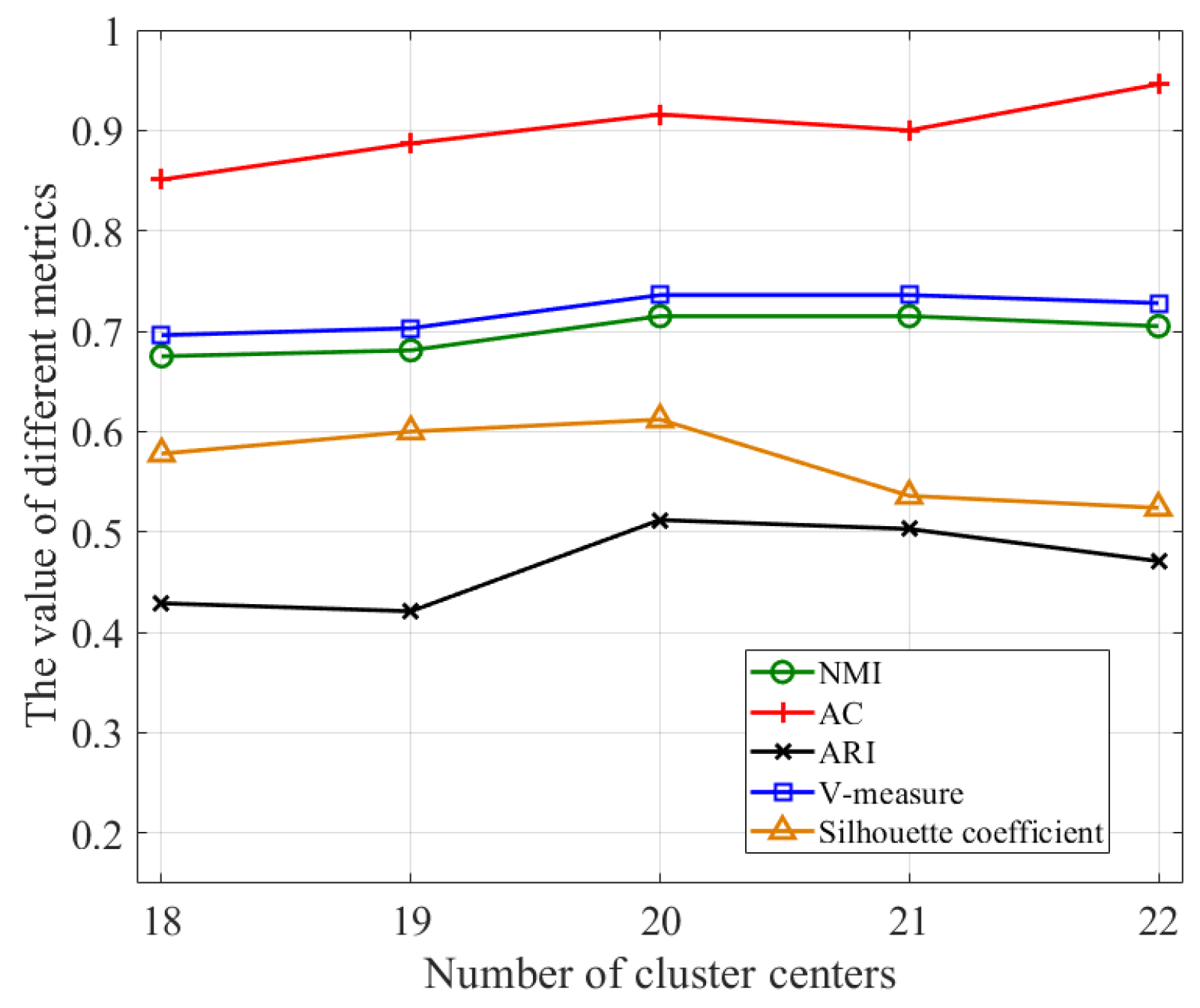
5.2.4. The Influence of the Uncertainty in the Number of Categories on NTC Performance

For unsupervised clustering, there is an inevitable disadvantage, that is, it is difficult to determine the appropriate number of clusters in advance, resulting in a low clustering quality. The key to obtain a good clustering effect is to determine the optimal number of clusters. Therefore, this paper used the elbow method and the silhouette coefficient method to determine the optimal number of clusters. As a low-complexity linear dimensionality reduction method, the PCA algorithm is suitable for quickly determining the range of the optimal number of clusters in this paper. The objective function of k-means clustering is the squared sum of the distance between the sample and the center point, also known as the distortion. For a cluster, the lower the distortion, the closer the samples in the cluster are. The higher the distortion, the farther the samples in the cluster are. The distortion of samples decreases with the increase in clustering categories. However, if the data of each class of samples are very different, when the clustering class is close to the real class, the distortion is greatly reduced, and then tend to be flat. This turning point is considered as a point with good clustering performance. Based on this indicator, multiple k-means models were trained, and different k-values (cluster center) were selected for comparison, as shown in Figure 8.

When $k=20$, the distortion is greatly improved, and the maximum curvature value appears. For a sample set, its silhouette coefficient is the average value of all sample silhouette coefficients. The closer the distance between samples of the same category, the farther the distance between samples of different categories, and the higher the score, the better the classification effect. As can be seen from Figure 9, when $k=18$ and $k=20$, the silhouette coefficient has a high peak value. Combined with the elbow method diagram, when $k=20$, the average distortion is relatively small, and the trend is gentle. Therefore, $k=20$ can be considered as the best number of clusters.

After roughly determining the number of clusters, we verified the reliability of the proposed method. When $k=\left\{5,10,15,20,25\right\}$, the DC-CAAE model proposed in this paper was used for training. It can be seen from Figure 10 that when $k=20$, the accuracy of the model tends to be stable and the highest, which is consistent with the guess above. To further determine the specific values of the cluster, on the basis of Figure 10, we expanded the analysis to around $k=20$. Five points, $k=\left\{18,19,20,21,22\right\}$, were chosen for the demonstration. The experimental results are shown in Figure 11.

When $k=22$, the accuracy of the clustering is slightly improved compared to when $k=20$. The reasons for this situation are as follows: when the number of clusters is smaller than the real sample category, the number of cluster centers is small; hence, the samples of the additional categories will inevitably converge to other categories, resulting in too large a distance between the same category of samples. When the number of clusters is greater than the real sample category, the number of cluster centers is large, hence the same type of samples will be divided into multiple categories. However, this does not affect the evaluation of the clustering accuracy, and even the accuracy will be improved compared with the actual number of clusters. However, on the whole, when the cluster category is 20, the five evaluation indexes are relatively stable, and $k=20$ has the best performance.

6. Conclusions

Aiming at the low accuracy of unsupervised learning classification in security applications of the IoT, this paper proposed an unsupervised NTC method using adversarial training and deep clustering under complicate IoT environments. The introduction of the CAAE for reducing the dimension of features can avoid the huge computational cost caused by the high complexity of high-dimensional original network traffic data features. The DC cell is the key building block of our model because it not only adapts the extracted features to the clustering network but also has a lower computational overhead than the CAAE model. In the multiclassification task, we gave a method to optimize the distance between clusters and within clusters through the joint analysis of cluster error and feature learning. It also indicated that the number of clusters could be determined by the elbow method and silhouette coefficient method when the sample class was unknown. The experimental results provided showed that the model not only had good network traffic classification performance but could also run efficiently in an unsupervised environment, greatly saving the cost of labeling. Therefore, our proposed unsupervised NTC method can provide a feasible solution for real application scenarios of the IoT and also provide a new idea to improve the unsupervised clustering accuracy under complex data conditions. In the future, we plan to study the detection of abnormal network traffic, that is, to identify and detect unknown malicious attacks in intrusion detection systems and to deploy them experimentally in a real industrial IoT dataset.

References

1. Nguyen, D.C.; Ding, M.; Pathirana, P.N.; Seneviratne, A.; Li, J.; Niyato, D.; Dobre, O.A.; Poor, H.V. 6G internet of things: A comprehensive survey. IEEE Internet Things J. 2022, 9, 359–383. [Google Scholar] [CrossRef]
2. Guo, F.; Yu, F.R.; Zhang, H.; Li, X.; Ji, H.; Leung, V.C.M. Enabling massive IoT toward 6G: A comprehensive survey. IEEE Internet Things J. 2021, 8, 11891–11915. [Google Scholar]
3. Lampe, B.; Meng, W. A survey of deep learning-based intrusion detection in automotive applications. Expert Syst. Appl. 2023, 221, 119771. [Google Scholar]
4. Li, W.; Meng, W.; Kwok, L.F. Surveying Trust-Based Collaborative Intrusion Detection: State-of-the-Art, Challenges and Future Directions. IEEE Commun. Surv. Tutor. 2022, 24, 280–305. [Google Scholar]
5. Zhou, X.; Liang, W.; Li, W.; Yan, K.; Shimizu, S.; Wang, K. Hierarchical adversarial attacks against graph-neural-network-based IoT network intrusion detection system. IEEE Internet Things J. 2022, 9, 9310–9319. [Google Scholar]
6. Popoola, S.I.; Ande, R.; Adebisi, B.; Gui, G.; Hammoudeh, M.; Jogunola, O. Federated deep learning for zero-day botnet attack detection in IoT edge devices. IEEE Internet Things J. 2022, 9, 3930–3944. [Google Scholar] [CrossRef]
7. Nguyen, T.; Armitage, G. A survey of techniques for internet traffic classification using machine learning. IEEE Commun. Surv. Tutor. 2008, 10, 56–76. [Google Scholar] [CrossRef]
8. Dias, K.L.; Pongelupe, M.A.; Caminhas, W.M.; Errico, L. An innovative approach for real-time network traffic classification. Comput. Netw. 2019, 158, 143–157. [Google Scholar] [CrossRef]
9. Pasyuk, A.; Semenov, E.; Tyuhtyaev, D. Feature selection in the classification of network traffic flows. In Proceedings of the International Multi-Conference on Industrial Engineering and Modern Technologies (FarEastCon), Vladivostok, Russia, 1–4 October 2019; pp. 1–5. [Google Scholar]
10. Moore, A.W.; Zuev, D. Internet traffic classification using bayesian analysis techniques. ACM Sigmetrics Perform. Eval. Rev. 2005, 33, 50–60. [Google Scholar] [CrossRef]
11. Min, E.; Guo, X.; Liu, Q.; Zhang, G.; Cui, J.; Long, J. A Survey of Clustering With Deep Learning: From the Perspective of Network Architecture. IEEE Access 2018, 6, 39501–39514. [Google Scholar] [CrossRef]
12. Karagiannis, T.; Broido, A.; Faloutsos, M.; Klaffy, K. Transport Layer Identification of P2P Traffic. In Proceedings of the 4th ACM SIGCOMM Conference on Internet Measurement (IMC 2004), Taormina Sicily, Italy, 25–27 October 2004; pp. 121–134. [Google Scholar]
13. Dusi, M.; Gringoli, F.; Salgarelli, L. Quantifying the accuracy of the ground truth associated with Internet traffic traces. Comput. Netw. 2011, 55, 1158–1167. [Google Scholar] [CrossRef]
14. Dreger, H.; Feldmann, A.; Mai, M.; Paxson, V.; Sommer, R.R. Dynamic application layer protocol analysis for network intrusion detection. In Proceedings of the USENIX Security Symposium, Vancouver, BC, Canada, 31 July–4 August 2006; pp. 257–272. [Google Scholar]
15. Madhukar, A.; Williamson, C. A longitudinal study of P2P traffic classification. In Proceedings of the 14th IEEE International Symposium on Modeling, Analysis, and Simulation, Monterey, CA, USA, 11–14 September 2006; pp. 179–188. [Google Scholar]
16. Paxson, V. Empirically derived analytic models of wide-area TCP connections. IEEE/ACM Trans. Netw. 1994, 2, 316–336. [Google Scholar] [CrossRef]
17. Sadeghzadeh, A.M.; Shiravi, S.; Jalili, R. Adversarial network traffic: Towards evaluating the robustness of deep-learning-based network traffic classification. IEEE Trans. Netw. Serv. Manag. 2021, 18, 1962–1976. [Google Scholar] [CrossRef]
18. Ma, W.; Qi, C.; Zhang, Z.; Cheng, J. Sparse channel estimation and hybrid precoding using deep learning for millimeter wave massive MIMO. IEEE Trans. Commun. 2020, 68, 2838–2849. [Google Scholar] [CrossRef]
19. Zhao, R.; Gui, G.; Xue, Z.; Yin, J.; Ohtsuki, T.; Adebisi, B.; Gacanin, H. A novel intrusion detection method based on lightweight neural network for internet of things. IEEE Internet Things J. 2022, 9, 9960–9972. [Google Scholar]
20. Ning, J.; Gui, G.; Wang, Y.; Yang, J.; Adebisi, B.; Ci, S.; Haris, G.; Gacanin, H. Malware traffic classification using domain adaptation and ladder network for secure industrial internet of things. IEEE Internet Things J. 2022, 9, 17058–17069. [Google Scholar]
21. Huang, P.; Huang, Y.; Wang, W.; Wang, L. Deep embedding network for clustering. In Proceedings of the 22nd International Conference on Pattern Recognition, Stockholm, Sweden, 24–28 August 2014; pp. 1532–1537. [Google Scholar]
22. Li, P.; Chen, Z.; Yang, L.T.; Gao, J.; Zhang, Q.; Deen, M.J. An improved stacked auto-encoder for network traffic flow classification. IEEE Netw. 2018, 32, 22–27. [Google Scholar]
23. Shah, S.; Koltun, V. Deep Continuous Clustering. 2018. Available online: https://arxiv.org/abs/1803.01449 (accessed on 5 March 2018).
24. Srivastava, R.; Greff, K.; Schmidhuber, J. Training very deep networks. In Proceedings of the Neural Information Processing Systems (NIPS), Red Hook, NY, USA, 7–12 December 2015; pp. 2377–2385. [Google Scholar]
25. Thies, J.; Alimohammad, A. Compact and low-power neural spike compression using undercomplete autoencoders. IEEE Trans. Neural Syst. Rehabil. Eng. 2019, 27, 1529–1538. [Google Scholar] [CrossRef] [PubMed]
26. Wang, W.; Zhu, M.; Zeng, X.; Ye, X.; Sheng, Y. Malware traffic classification using convolutional neural network for representation learning. In Proceedings of the International Conference on Information Networking (ICOIN), Da Nang, Vietnam, 11–13 January 2017; pp. 712–717. [Google Scholar]
27. Ren, Y.; Pu, J.; Yang, Z.; Li, G.; Pu, X.; Yu, P.; He, L. Deep Clustering: A Comprehensive Survey. 2022. Available online: https://arxiv.org/abs/2210.04142 (accessed on 9 October 2022).
28. Hoang, D.H.; Nguyen, H.D. Detecting anomalous network traffic in IoT networks. In Proceedings of the International Conference on Advanced Communication Technology (ICACT), PyeongChang, Republic of Korea, 17–20 February 2019; pp. 1143–1152. [Google Scholar]
29. Peng, X.; Xiao, S.; Feng, J.; Yau, W.-Y.; Yi, Z. Deep subspace clustering with sparsity prior. In Proceedings of the International Joint Conferences on Artificial Intelligence Organization (IJCAI), New York, NY, USA, 9–15 July 2016; pp. 1925–1931. [Google Scholar]
30. Yao, R.; Liu, C.; Zhang, L.; Peng, P. Unsupervised anomaly detection using variational auto-encoder based feature extraction. In Proceedings of the IEEE International Conference on Prognostics and Health Management (ICPHM), San Francisco, CA, USA, 17–20 June 2019; pp. 1–7. [Google Scholar]
31. Yang, B.; Fu, X.; Sidiropoulos, N.D.; Hong, M. Towards K-means-friendly spaces: Simultaneous deep learning and clustering. In Proceedings of the 34th International Conference on Machine Learning (ICML 2017), Sydney, Australia, 6–11 August 2017; pp. 3861–3870. [Google Scholar]
32. Guo, X.; Liu, X.; Zhu, E.; Zhu, X.; Li, M.; Xu, X.; Yin, J. Adaptive self-paced deep clustering with data augmentation. IEEE Trans. Knowl. Data Eng. 2020, 32, 1680–1693. [Google Scholar] [CrossRef]
33. Rabiner, L. Combinatorial optimization: Algorithms and complexity. IEEE Trans. Acoust. Speech Signal Process. 1984, 32, 1258–1259. [Google Scholar] [CrossRef]
Figure 1. Flowchart of unsupervised-learning-aided NTC method.
Futureinternet 15 00298 g001
Figure 2. The detailed process of data preprocessing.
Futureinternet 15 00298 g002
Figure 3. The model framework of the proposed DC-CAAE method. The model is divided into two steps, CAAE and DC. First, the CAAE network is used to preliminarily train the feature extractor, then DC constraints are added to fine-tune the feature extractor so that the extracted features are oriented toward clustering tasks.
Futureinternet 15 00298 g003
Figure 4. The framework of the proposed CAAE method.
Futureinternet 15 00298 g004
Figure 5. The framework of the deep clustering algorithm.
Futureinternet 15 00298 g005
Figure 6. Convergence trend of overall cluster loss during training.
Futureinternet 15 00298 g006
Figure 7. t-SNE feature visualizations for different clustering algorithms. (a) CAE; (b) CVAE; (c) CAAE; (d) DC-CAE; (e) DC-CVAE; (f) DC-CAAE.
Futureinternet 15 00298 g007
Figure 8. The change in average distortion at different cluster centers.
Futureinternet 15 00298 g008
Figure 9. The change in silhouette coefficient at different cluster centers.
Futureinternet 15 00298 g009
Figure 10. Performance of the DC-CAAE model at k = 5 , 10 , 15 , 20 , 25 .
Futureinternet 15 00298 g010
Figure 11. Performance of the DC-CAAE model at k = 18 , 19 , 20 , 21 , 22 .
Futureinternet 15 00298 g011