Evaluation of Machine Learning Algorithms in the Classification of Multispectral Images from the Sentinel-2A/2B Orbital Sensor for Mapping the Environmental Dynamics of Ria Formosa (Algarve, Portugal)

Abstract

With the growing availability of remote sensing orbital spatial data, the applications of machine learning (ML) algorithms have been leveraging the field of process automation in image classification. The present work aimed to evaluate the precision and accuracy of ML algorithms in the classification of Sentinel 2A/2B images from an area of high environmental dynamics, such as Ria Formosa (Algarve, Portugal). The images were submitted to classification by groups of ML algorithms such as the Support Vector Machine (SVM), Random Forest (RF), K-Nearest Neighbors (KNN), and Decision Tree (DT). The Orfeo Toolbox (OTB) open-source programming package made the algorithms available. Ten samples were collected for each of the 14 land use and cover classes in the Ria Formosa area, totaling 140 samples. Of these, 70% were for training and 30% for validating the classification. The evaluation metrics used were the class discrimination measures: Recall (R), the Global Kappa Index (k), and the General Accuracy Index (OA). The results showed that the KNN and DT algorithms demonstrated a greater discrimination capacity for most classes (. SVM and RF significantly improved class discrimination when using larger samples for training. Merging the classified images significantly improved the classification accuracy, ranging from 71% to 81%. This evaluation made it possible to define sets of ML algorithms sensitive to change detection for mapping and monitoring dynamic environments.

1. Introduction

Orbital remote sensing images are being increasingly improved and more easily made available due to the efforts of space agencies in launching new generations of satellites and the free access to pre-processed or corrected images in repositories or hubs in the world’s computer networks. This recent innovation has allowed for a range of applications for monitoring and mapping terrestrial and marine resources [1]. With this, image classification is the topic that has given more fantastic support to this theme, being one of the largest fields of applications of remote sensing [2].

Remote sensing image classification algorithms are based on the statistics of sets of pixels sampled in the images to obtain the mapping classes of interest. Although several techniques have different statistical forms of image classification, many algorithms have been developed in the last two decades [3]. However, there are still gaps in understanding their performances and efficiency regarding the number of samples and classes required to produce more accurate mappings.

In any case, this is explained by the consensus that remote sensing image classification techniques, as products, evolve towards increased spatial and spectral resolution, and depending on the diversity of mapping classes and their mixtures, the traditional algorithms are not as effective in distinguishing with the same accuracy the classes detected in the images [1,4]. In addition, they need more sampling or processing interactions, such as greater adjustments or composition transformations, or spectral band indices, which highlight the targets or classes of interest to enable greater accuracy [5].

Recently, image classification techniques by algorithms based on machine learning (ML) are opening new perspectives on how data are conceived and analyzed by sets of algorithms that can infer in their logical functions’ categorization concepts arising from the nature of the data. Supervised ML algorithms have become a new frontier in the modeling and classification of remote sensing images due to their ease of implementation and process automation.

In the same way that traditional algorithms are categorized, ML image classification algorithms are classified into supervised classifiers (when the user performs a previous step of collecting samples for training on the image and uses a classifier to obtain the mapping classes) and unsupervised (when the user directly uses a classifier to identify the mapping classes later).

This work aimed to investigate the application of supervised machine learning algorithms in the classification of pre-processed images provided by the Sentinel 2A/2B Satellite to understand its classification performance (efficacy and accuracy) in levels of number, shape, and size of samples for training or learning.

The remote sensing images used in this study comprised an area of a dynamic environment, such as the coastal barrier island system of Ria Formosa, Algarve, Portugal. This perspective of the application of ML algorithms for the image classification of areas of dynamic environments and of great environmental interest aimed to list or score algorithms that best apply the nature of data inherent to these environments, as they can potentially be used in monitoring the responses to climate change in environments that have a high diversity of land use and occupation.

2. Materials and Methods

2.1. Study Area

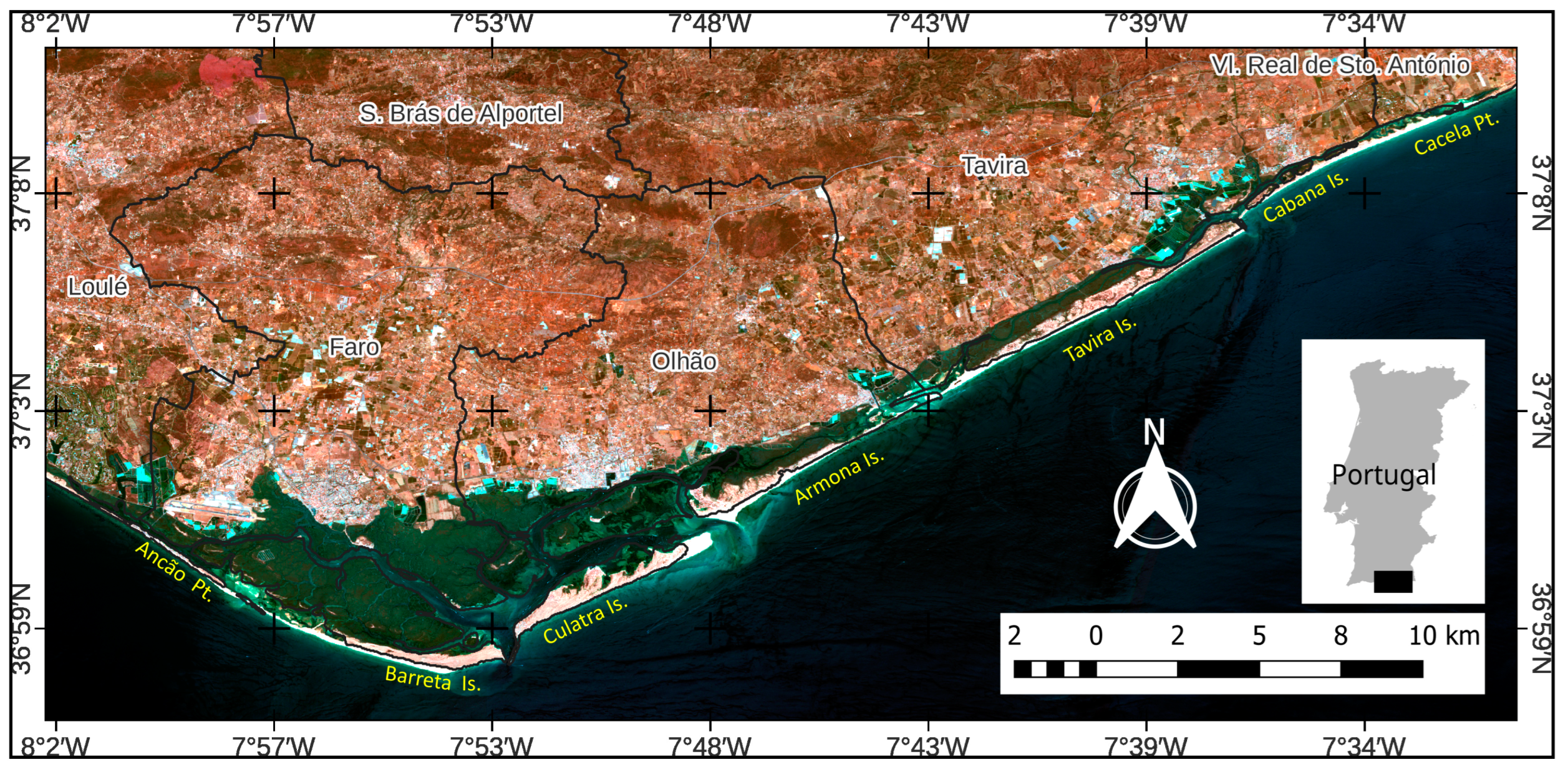
The Ria Formosa is a subtropical wetland that is in the southeastern coastal region of Portugal between the parallels of 36°55′ N and 37°10′ N and between the meridians of 8°10′ W and 07°30′ W (Figure 1). It consists of a system of sandy barrier islands that extends for 50 km, from west to east, composed of five islands called Barreta, Culatra, Armona, Tavira, and Cabanas, which are delimited by six tidal channels. At its end, it is delimited by two peninsulas called Ancão and Cacela, which connect to the mainland and are formed by extensive sandy spits [6,7,8].

The Köppen classification describes the climate as hot-summer Mediterranean (CSa), with an average temperature of 18.0 °C. The hottest months are from June to September, with an average temperature of 24.2 °C, and the coldest are from December to March, with an average temperature of 12.0 °C. Summer has much less rainfall than winter, and the average annual precipitation is 511.6 mm, with the period from June to August having little or no rain and October to January, the rainiest, with an average rainfall of 370 mm [9].

The average hourly wind speed experiences significant seasonal variation throughout the year. The windiest season of the year runs from October to April, with average wind speeds above 18.4 km/h, and with December being the month with the strongest winds at 20.7 km/h. The weakest winds go from May to September with speeds of 15.9 km/h. The prevailing wind direction is east in summer and north in winter. It has an average of 3428.54 h of sunshine per year, with July having the most daily hours of sun, with an average of 12.41 h/day, and the lowest, January, with an average of 6.57 h/day [9].

The tides are semi-diurnal and reach the limit of 3.2 m in spring tides, forming a meso-tidal regime [8]. Inside the lagoon, the muddy and sandy-muddy plains are vegetated by two predominant species: Spartina maritime and Sarcocornia fruticosa, which constitute the salt marsh environments [7]. The marine grasses of Zostera noltii colonize the muddy plains in their inter-tidal zone. In the infra-tidal areas, they are dominated by the aquatic grasses Cymodocea nodosa, Zostera marina, and Zostera noltii [7].

The supply of marine water in the Ria Formosa is more significant and predominant, as the rivers (Seco, Gilão, Ribeiras of Almargem, Lacém, Cacela, and others) that flow into the lagoon system are seasonal due to low local rainfall, with a torrential regime only in the more concentrated rainy season.

The municipalities located on the Ria Formosa’s borders are Loulé, Faro, Olhão, Tavira, and Vila Real de Santo Antonio, and comprise a population of 230,942 inhabitants [10]. The main economic activities developed in the Ria Formosa region are tourism, ecotourism, aquaculture, fishing, natural conservation, navigation, port activities, agriculture, salt extraction, and sediment mining, among others [6]. Such actions have modified the natural environment due to the construction of dikes, marinas, channel embankments, dredging, discharges of urban-industrial effluents, and urbanization of barrier islands and on the banks of lagoons [11].

Since 1978, the Ria Formosa has been considered a natural reserve. Since 1987, following Decree-Law 373/87 on 9 December, the Ria Formosa has been constituted as a Natural Park due to its environmental fragility and great historical importance, both cultural and economic [7].

2.2. Selection of Pre-Processed Data

Due to the focus of this work being the implementation of ML image classification algorithms to evaluate their use in the detection of environments (classes) of intense changes, as is the case in the Ria Formosa Barrier Islands System, the input images purposely comprised different situations’ climate and hydrodynamics, referring to the winter and summer periods, and spring and neap tides. These climate and circulation conditions inferred scenarios of more extreme or diverse environmental variables (e.g., increased discharges, current speeds, migration of bars and dunes, progradation and retrogradation of the coastline and sandy strips, changes in depth channels, and flood levels of marshy areas).

With this, Sentinel 2A and 2B satellite images were collected from the European Space Agency repository, Open Access Hub (https://scihub.copernicus.eu/, accessed on 3 march 2022) at pre-processing level 2A, which refers to image data with atmospheric correction by converting top-of-atmosphere-TOA reflectance to bottom-of-atmosphere-BOA reflectance. They also refer to images that have a geometric correction (UTM coordinates/Zone 29 N, Datum WGS 84) and pixel spatial resolution of 10 m for bands 02 (490 nm-blue), 03 (560 nm, green), 04 (665 nm, red), and band 08 (842 nm, near-infrared); 20 m for bands 05, 06, 07, 8 A (705 nm, 740 nm, 783 nm, 865 nm, edge red), and bands 11 and 12 (1610 nm, 2190 nm, shortwave infrared). Bands B01 (443 nm, aerosol), B09 (940 nm, water vapor), and B10 (1375 nm, cirrus), with a spatial resolution of 60 m, since they are used for atmospheric corrections, were not added as spectral data in this work. The radiometric resolution of this sensor’s bands was 12 bits (4096 gray levels) per pixel [12].

The total coverage of the Ria Formosa region was given by a set of 04 scenes of orbital images from Sentinel 2A and 2B. In the selection of the respective images, the dates and times of imaging were taken according to the hourly forecasts of the tide tables of the Commercial Port of Faro/PT, with the collected scenes referring to the summer and winter seasons and the tide heights in the quadrature and syzygy periods (

Table 1. Point/orbit of Sentinel Scenes 2A and 2B according to seasonality and tidal amplitude.

Scenes	Tidal Amplitude	Seasons	Periods	Date
L2A_T29SNA_A023229_20210817T112113	1.4 m	summer	quadrature	17 August 2021
L2A_T29SNB_A023229_20210817T112113
L2A_T29SPA_A023229_20210817T112113
L2A_T29SPB_A023229_20210817T112113
L2A_T29SNA_A032209_20210822T112449	2.9 m	summer	syzygy	22 August 2021
L2A_T29SNB_A032209_20210822T112449
L2A_T29SPA_A032209_20210822T112449
L2A_T29SPB_A032209_20210822T112449
L2A_T29SNA_A034354_20220119T112449	2.4 m	winter	syzygy	19 January 2022
L2A_T29SNB_A034354_20220119T112449
L2A_T29SPA_A034354_2022019T112449
L2A_T29SPB_A034354_20220119T112449
L2A_T29SNA_A034640_20220208T113014	1.1 m	winter	quadrature	8 February 2022
L2A_T29SNB_A034640_20220208T113014
L2A_T29SPA_A034640_20220208T113014
L2A_T29SPB_A034640_20220208T113014

).

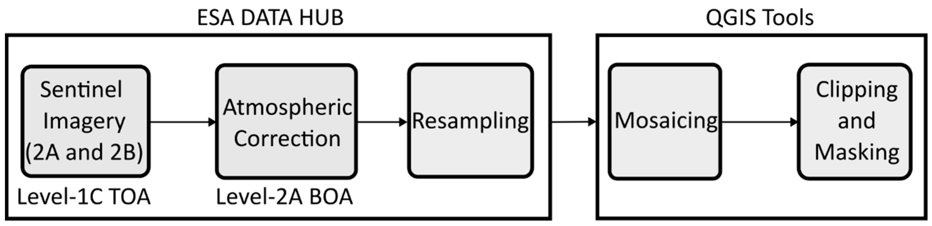
The mosaic of these scenes was obtained by the image fusion algorithm (Gdal_ merge.py) using QGis v. 3.22.16, a free software used in this work because it is an open-source project [13] that integrates Gdal and GRASS algorithms. Each scene mosaic produced and resampled to a spatial resolution of 10 m was subjected to a Boolean mask (0: outside the area of interest and 1: area of interest), using the GRASS algorithm “r.mask.rast” to contextualize only data from Ria Formosa and its surroundings, eliminating distant areas from the data context as invalid data (NULL DATA) (Figure 2).

2.3. Image Classifiers Based on ML Algorithms

The groups of ML algorithms addressed in this work were the Support Vector Machine (SVM), Random Forest (RF), K-Nearest Neighbors (KNN), and Decision Tree (DT). All ML models were implemented using the Orfeo ToolBox (OTB) v. 8.1.1, an open-source programming package project that integrates a variety of ML algorithms [14], and interfaces as a processing tool in the GIS environment QGis v.3.22.16 [13].

The Support Vector Machine (SVM) algorithm is one of the most traditional supervised ML classifier algorithms. The SVM classifier uses different planes in (n-dimensional) space to divide data points (pixels) (i.e., supposing two, linearly separable classes, the training objective is to determine a hyperplane in the feature space, which has the maximum distance from the nearest samples of both classes) [15]. Its performance and accuracy depend on selecting the hyperplane and the kernel parameter, which will produce a pixel classification model based on the training data or samples that can accurately predict class labels from the test data [3]. The source used in the OTB package comes from the Libsvm ML and OpenCV ML libraries [14].

The SVM is an easy-to-implement algorithm because it has practically two adjustment hyperparameters, such as Parameter C, for a penalty, and the Gamma Coefficient for the Polynomial, Radial Basis, and Sigmoidal kernel functions. The parameters used in this work for the SVM classifier were using a “linear kernel” type function for faster computational performance, with permission to develop a training model that accepted imperfections in the separation of classes, with the parameters C = 1 and Gamma = 1. The decision cost parameter (Nu = 0.5) remained as default, between the range of 0 to 1, to allow an intermediate classification between rigid (Nu = 0) and flexible (Nu = 1) types.

The ML Random Forest (RF) classifier is another algorithm widely used in pixel classification which is based on methods of generating an infinity of Decision Trees by joint learning and which evolves to a combination of these trees to obtain better ranking performance by averaging predictions [15,16]. Each Decision Tree is realized as a tree structure consisting of two types of nodes: decision and leaf nodes [15]. All trees are trained with the same parameters but using different sets of training samples. These sets are generated from the original training set using the “bootstrap” procedure; for each training set, the same number of vectors as the original set (=N) is randomly selected. Vectors are chosen with a replacement; some vectors will occur more than once, and some will be absent. Not all variables are used to find the best split at each node of each trained tree, but a random subset of them. Each node generates a new subgroup, with its size fixed for all nodes and trees.

The hyperparameters used by the RF algorithm to generate the training model were a maximum of 100 trees per forest (n estimators = 100) and, in each tree, a maximum of combinations of up to 5 trees (max depth number tree = 5) to generate each tree, with a minimum of 10 samples used to split each internal node (min_samples_split = 10), to reach the possible values of grouping categories that generate nodes with a minimum of 10 branches to the left and right (min samples leaf = 10) as some clustering categories (K <= cat clusters). These values were adjusted by default in the OTB package to avoid under or overadjustments “under and overfitting” and, by default, not allowing any of the constructed trees to be pruned.

The K-Nearest Neighbor (KNN) algorithm is among the simplest ML algorithms. It is a method for classifying objects based on training samples that make it possible to generate vectors that predict the statistical characteristics of approximate or neighboring pixels. The training process for this algorithm just consists of caching all the training samples and generating vectors obtained by the class labels of the training images as integer values. In the classification process, the set of unlabeled pixels is simply assigned to the class label as a function of the nearest K (constant) vector by the Euclidean metric, using the vote calculated by the weighted sum of the distance between the nearest neighbors [4,17]. In the case of OTB, a single adjustment parameter is the number of pixels (K) near neighbors for use in image classification, with the value of K = 32 being used as the default.

The Decision Tree (DT) classifier [18,19] is an inductive learning algorithm that generates a classification tree using the training data/sample. It is based on the “divide and conquer” strategy. It mainly consists of three parts: partitioning the nodes, finding the terminal nodes, and allocating the class label to the terminal nodes. It uses a hierarchical rule with high-dimensional data arranged in a tree. When the Decision Tree is built, many branches reflect noise in the training pattern, so pruning the tree tries to identify and remove such branches and improve the classification accuracy.

The hyperparameters used by OTB as the default for the DT algorithm are as follows: (max depth tree = 5), that is, the training algorithms try to divide a node while the generation of trees is less than 5 trees; (minimum samples count = 10), which refers to a minimum number of samples to cut a node; and (max_categories = 10), which is the maximum number of possible values of a categorical variable in k-clusters to find a suboptimal division. In this case, if a discrete variable that the training procedure tries to divide takes more than max_categories values, it may take an extended processing time because the algorithm generates exponentially many combinations to obtain an estimate that best represents each subset of samples. Instead, in this case, many Decision Tree engines (including ML) try to find a suboptimal split by grouping all samples into max_categories clusters, i.e., some categories end up being merged.

In OTB Tool Box v.8.1.1, each ML algorithm has common steps to normalize the data between the scene bands. The following steps give the stages: the 1st calculates the statistics for each image (band); 2nd calculates the sampling rate for each image; 3rd selects the positions of the samples for each image; 4th extracts statistical measurements from the samples for each image; 5th trains the model from the number of samples per class and their geometry (which can be points, lines, and polygons), with each feature having an integer number that identifies the class, and these between themselves the identical amounts of samples; 6th generates the classification model based on the functions and parameters of the selected classification algorithm; 7th generates the confusion matrix and the evaluation metrics.

The evaluation metrics generated in the training and validation phases of the classifier model by the OTB for each class, and used in this work, were the Recall (R) measures or True Positive Rate ([TPR] = Discrimination Sensitivity), which were calculated by Equation (1).

$$\left(TPR\right)=\frac{\left(TP\right)}{\left(TP\right)+\left(FN\right)}$$

(1)

where (TP) = True Positives, and (FN) = False Negatives; and Precision (P) is given by Equation (2).

$$\left(P\right)=\frac{\left(TP\right)}{\left(TP\right)+\left(FP\right)}$$

(2)

where (FP) = False Positives; and F1-Score (a precision measure that represents the harmonic mean between Precision (P) and Recall (R)) is given by Equation (3).

$$\left(F1\text{-}Score\right)=2\times \frac{\left(P\right)\times \left(TPR\right)}{\left(P\right)+\left(TPR\right)}$$

(3)

The Global Kappa Index (K) and the Overall Accuracy Index (OA) were also generated using the Confusion Matrix obtained in the classification’s training and validation phases. The Global Kappa Index is acquired by the following Equation (4):

$$\left(K\right)=\frac{\left[\left(\mathsf{\Sigma }NP\right)\times \left(\mathsf{\Sigma }VP\right)\right]-\left[{\left(\mathsf{\Sigma }VP\right)}^2\times \mathsf{\Sigma }(FP\times FN)\right]}{\left[\left({\mathsf{\Sigma }NP}^2\right)\right]-\left[{\left(\mathsf{\Sigma }VP\right)}^2\times \mathsf{\Sigma }\left(FP-FN\right)\right]}$$

(4)

where (ΣNP) = sum of the number of validated and non-validated trained pixels of all classes as a reference, that is, the total number of samples in all classes; (ΣVP) = sum of the number of correctly classified pixels observed in all classes; [Σ(FP × FN)] = sum of the product of FP (False Positives) by FN (False Negatives) of each class.

The Overall Accuracy Index (OA) consisted of the number of correctly classified pixels observed in all classes (ΣVP), concerning the number of trained and validated pixels in all classes as a reference; that is, it was obtained from the total sums of the confusion matrix of the training and validation samples as reference classes, and between the unlimited sums of the estimated or observed classes after training each ML algorithm.

2.4. Preparation of Training Samples

The initial step for obtaining the training samples was the use of a set of image segmentation algorithms, which in themselves can be understood as “pre-classifiers” since they do not have defined classes at this processing stage, but the configuration of a vector coverage of polygons that delimit objects (sets of pixels or segments in images with similar spatial, spectral, and textural characteristics). Effective segmentation ensures greater classification accuracy [14].

In this work, the “mean-shift” segmentation algorithm was used in the “default” mode of the Orfeo ToolBox (OTB) v.8.1.1 programming package. This step belonged to the Object-Based Image Analysis (OBIA). The segmentation algorithm employed the “mean-shift” moving average method to divide images based on pixel variance. The resulting image was transformed into a cluster image of pixel allocation surfaces by obtaining the segments based on the similarity of pixel variance between the spectral bands. The algorithm was adjusted for a search window in a radius of 5 pixels and with a similarity tolerance of 15 pixels between the bands. The average weight and variance factor used was 0.5 to evaluate the similarity between the pixels of neighboring segments. These adjustments were the default type to provide a balance between the segments’ size and the variations of objects detected in the images.

In each set of Sentinel 2A and 2B scenes, the segmentation algorithm, as mentioned earlier, generated a vector file of polygons and a corresponding database, in which each polygon delimited on the image had an identity (id) resulting from the statistical delimitation of spectral arrangements between the bands and their respective shape of space objects on the ground. The process of collecting samples in the images was based on the selection of segments as samples in different classes of forms of land use and occupation, based on the interpretation of the images, to serve as training for the ML learning algorithms, thus determining the number of mapping classes to be implemented for generating classification models.

As a strategy for obtaining a single vector file of training samples that could be used to train all images in different periods, the vector files resulting from the segmentation process of each image were superimposed. From the intersection of each cover vector corresponding to each mosaic, a file of polygons of intersected training samples was generated, which made it possible to assume in this scenario that the selections of samples of spectrum arrangement and the landforms (morphologies) were similar and familiar, or more coherent, between the mosaics of scenes in all situations of neap and spring tides in the summer and winter season.

In another scenario, the segmentation vector files obtained from their respective images were also used as training samples by superimposing the centroids of the polygons of intersected samples, thus using the total area of the segment or selecting the entire segment to serve as a sample of training. This strategy was defined as a parameter for evaluating the performance of the classifier algorithms when they used training samples with a greater context, assuming that in this condition, the training samples constituted more significant variability given the environmental circumstances of the moment in which they were collected and obtained each image.

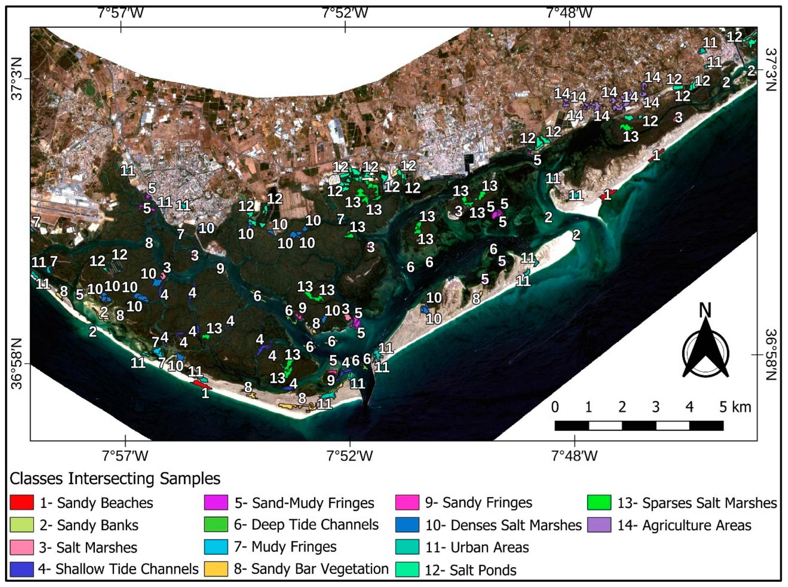
The interpreted classes corresponded in each mosaic of scenes to the typical morphologies of the Ria Formosa and were of interest for the monitoring of its environmental dynamics, as follows: 1—Sandy Beach, 2—Sand Bank, 3—Marisma (Salt Marsh), 4—Canal Shallow Tide, 5—Sandy-Muddy Fringe, 6—Deep Tide Channel, 7—Muddy Fringe, 8—Restinga Vegetation, 9—Sandy Fringes, 10—Dense Salt Marsh, 11—Urban Areas, 12—Salina (Salt Pond), 13—Sparse Marsh (Salt Marsh), and 14—Agricultural Areas (Figure 3).

Using an area size filter, polygons smaller than 1 ha (10,000 m²) were excluded, and ten polygons of each land use and occupation class were selected for sampling, obtaining a total of 140 samples. In each class, 07 samples were chosen for algorithm training (98 samples, or 70% of the set) and 03 for classification validation (42 samples, or 30% of the collection).

The classified images of each period by each classification algorithm were validated through a reference map (the vector file that constituted the intersected segments, and their training samples, such as the validation or test samples).

After generating the classified images, the validation metrics were evaluated by the Global Kappa Index (K), and Overall Accuracy (OA) was obtained by the validation confusion matrix in OTB v.8.1.1.

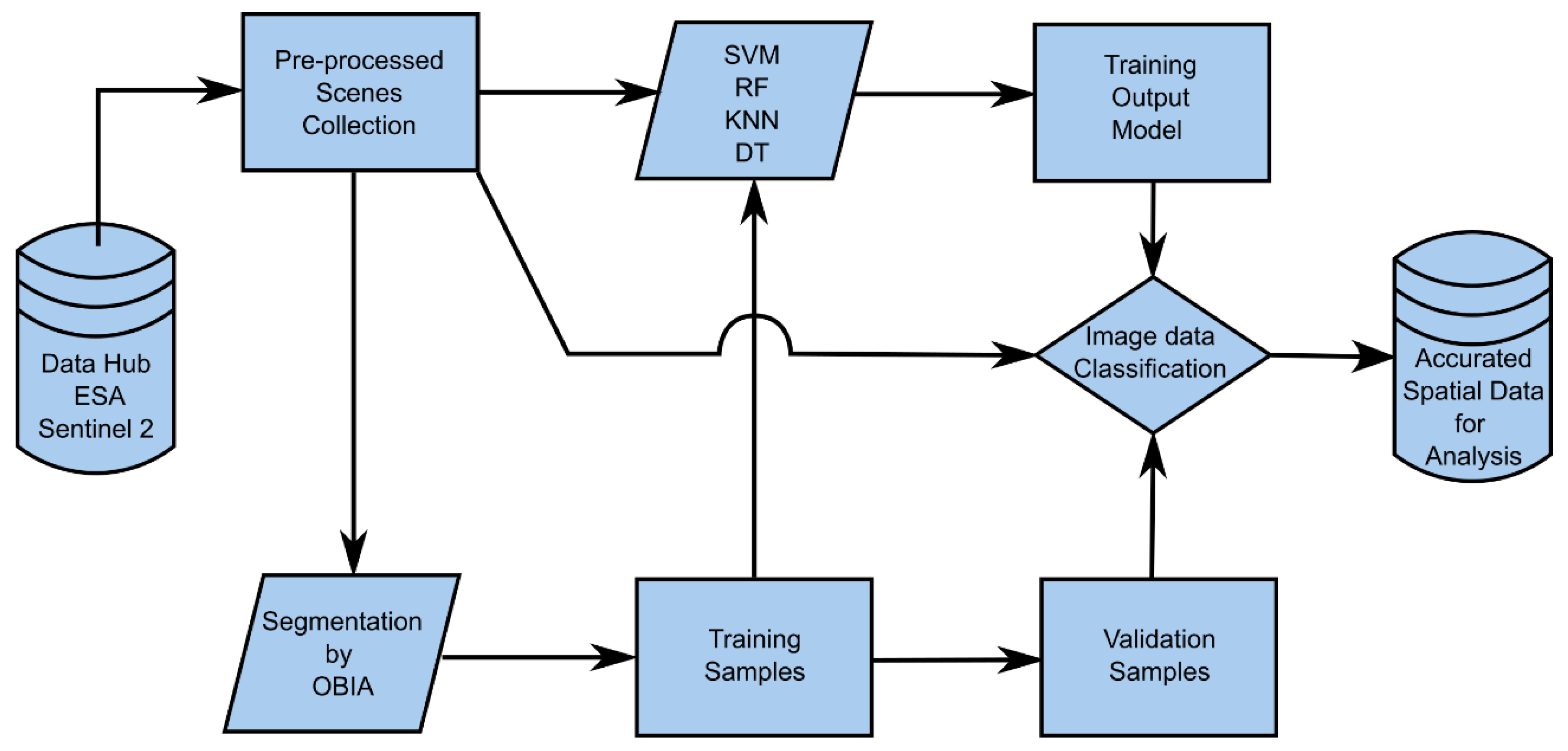
Still, as the purpose of this work was to plan a simplified tool (Figure 4) and more accurate environmental monitoring for the Ria Formosa to obtain more precise data that serve the analysis and environmental monitoring, the classes the classification algorithms were unable to discriminate by Recall (R) measures, or by the True Positive Rate (TPR), according to Tharwat’s classification sensitivity scale [20], were excluded. With this, the set of classified images of each training scenario was merged by a majority filter and subsequently submitted again for validation (Figure 4).

3. Results

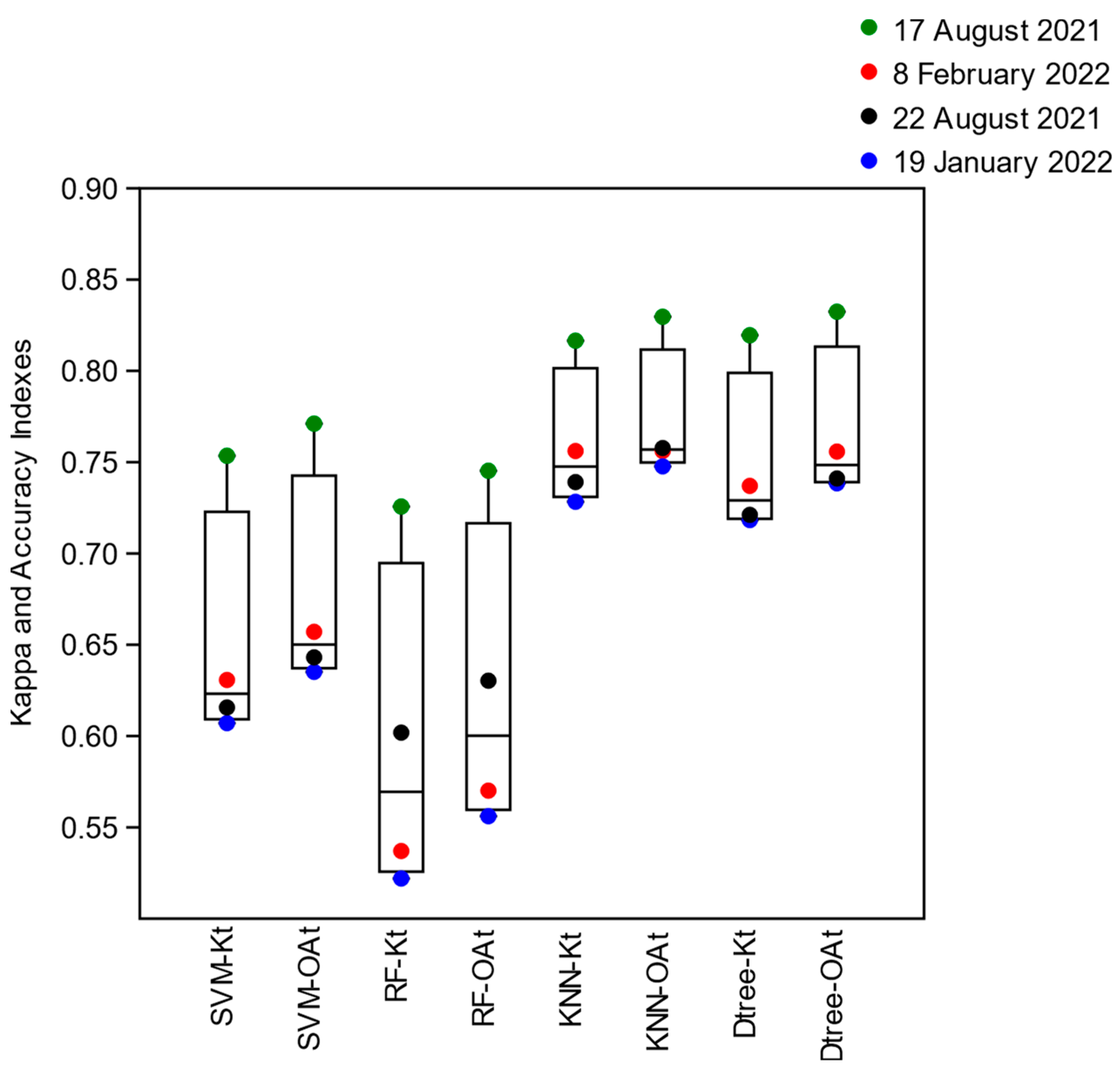
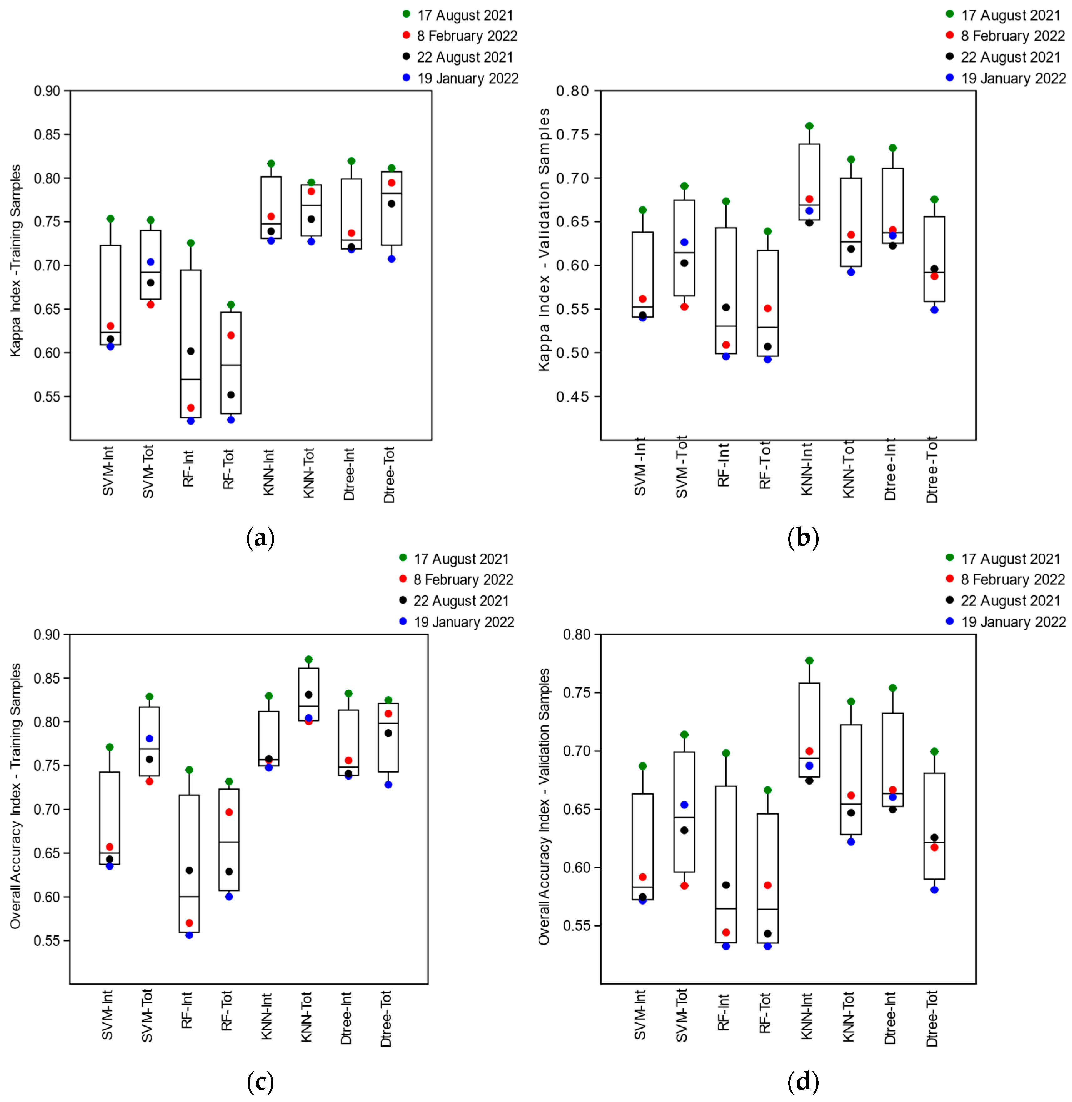
The evaluation of the training accuracy by the Global Kappa Indexes (Kt) obtained from the training confusion matrices of the SVM, Random Forest, KNN, and Decision Tree algorithms, when using the intersected segments as training samples (t), proved to be on average (͞x) more remarkable for the image of 17 August 2021 (͞x = 0.78, sd = 0.05) located in neap tide conditions (smaller tidal amplitude) in the summer season. The images from 8 February 2022 (͞x = 0.67, sd = 0.1), quadrature and winter, and 22 August 2021 (͞x = 0.67, sd = 0.07), and 19 January 2022 (͞x = 0.64, sd = 0.1) obtained under conditions of spring tide (greater tidal amplitude) in summer and winter, respectively, showed an approximate (͞x) of the Global Kappa Index (Kt) (Figure 5). The algorithms that obtained the highest Global Kappa (Kt) Indices for all images were KNN (͞x = 0.76, sd = 0.04) and Decision Tree (͞x = 0.75, sd = 0.05), and the lowest were SVM (͞x = 0.65, sd = 0.07), and Random Forest (͞x = 0.60, sd = 0.09) (Figure 5).

The average Overall Accuracy (OAt) Indices obtained in the training (t) of the classifier algorithms, using the intersected segments as samples, also demonstrated greater accuracy for the image of 17 August 2021 (͞x = 0.79, sd = 0.04) referring to the summer season under neap tide conditions. The Overall Accuracy (OAt) Indices of the image obtained in the summer at spring tide, 22 August 2021 (͞x = 0.69, sd = 0.07), and of the images obtained in the winter season at neap tide, 8 February 2022 (͞x = 0.68, sd = 0.09), and syzygy, 19 January 2022 (͞x = 0.67, sd = 0.09), were also situated with approximate means (͞x) (Figure 5). The algorithms that obtained the highest rates of Overall Accuracy (OAt) for all images were KNN and Decision Tree (͞x = 0.77, sd = 0.04), followed by SVM (͞x = 0.65, sd = 0.07) and Random Forest (͞x = 0.60, sd = 0.09) (Figure 5).

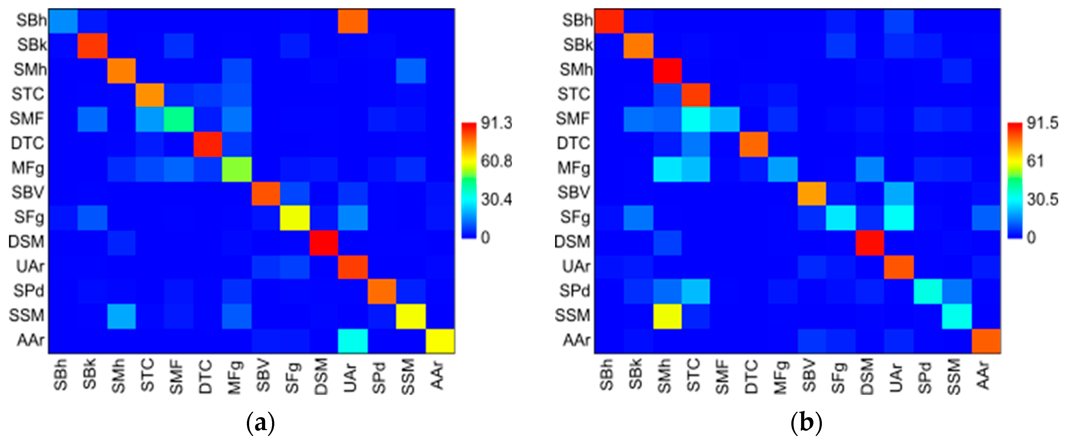
Comparing the confusion matrices of the algorithms by the classification sensitivity measure Recall (R), or the True Positive Rate (TPR), obtained in training using the intersection samples between segments of all images, demonstrated that the classifier algorithm SVM, on average (͞x) for all images, obtained the best Recall (R) for the classes “Dense Salt Marsh” (͞x = 0.91, sd = 0.02), “Deep Tide Channel” (͞x = 0.87, sd = 0.03), “Urban Areas” (͞x = 0.84, sd = 0.05), “Sandy Bank” (͞x = 0.84, sd = 0.08), “Sand Bar Vegetation” (͞x = 0.81, sd = 0.06), and “Salt Ponds” (͞x = 0.78, sd = 0.05), and the smallest Recall (R) for the classes “Sand-Muddy Fringe” (͞x = 0.43, sd = 0.33), “Sparse Salt Marshes” (͞x = 0.60, sd = 0.09), “Sandy Fringes” (͞x = 0.59, sd = 0.07), “Muddy Fringes” (͞x = 0.52, sd = 0.11), “Agriculture Areas” (͞x = 0.60, sd = 0.19), and “Sandy Beaches” (͞x = 0.16, sd = 0.07) (Figure 6a).

The Random Forest algorithm obtained the lowest Recall (R) concerning the other algorithms (mean “͞x” ranging from 0.19 to 0.34), except for the classes “Salt Marshes” (͞x = 0.91, sd = 0.06), “Dense Salt Marshes” (͞x = 0.89, sd = 0.03) “Sandy Beaches” (͞x = 0.86, sd = 0.04), “Shallow Tide Channel” (͞x = 0.85, sd = 0.15), “Urban Areas” (͞x = 0.81, sd = 0.05), and “Agriculture Areas” (͞x = 0.80, sd = 0.05) (Figure 6b). On the other hand, the highest recall averages were obtained by the KNN and Decision Tree algorithms in all images (average “͞x” ranging from 0.91 to 0.80) distributed in most classes, except in classes (average “͞x” ranging from 0.61 to 0.74) “Sand-Muddy Fringes”, “Sandy Fringes”, “Muddy Fringes”, and “Sparse Salt Marshes” (Figure 6c,d).

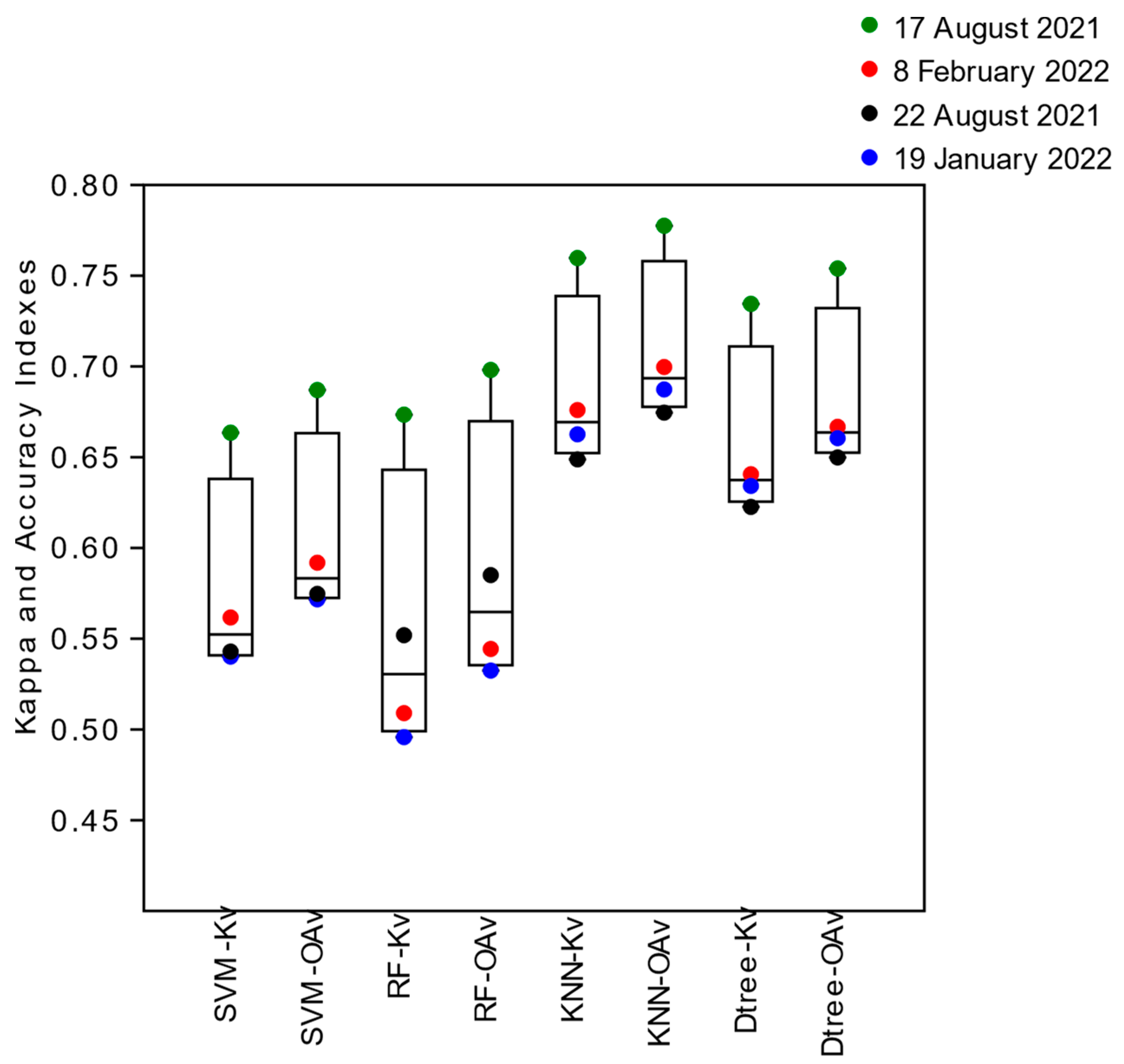
The average Global Kappa Indexes (Kv) obtained after the validation (v) of the images classified by the algorithms (SVM, Random Forest, KNN, and Decision Tree), which had the intersected segments as training samples, were shown larger for the image from 17 August 2021 (͞x = 0.71, sd = 0.05) of summer in quadrature conditions (lower tidal amplitude), and approximated for the images from 8 February 2022 (͞x = 0.60, sd = 0.08), referring to the winter season at neap tide, and 22 August 2021 (͞x = 0.59, sd = 0.05) and 19 January 2022 (͞x = 0.58, sd = 0.08) obtained under conditions of tide syzygy (greater tidal amplitude) in summer and winter, respectively (Figure 7). The algorithms that maintained the highest average Global Kappa Indexes (Kv) after image classification validation were KNN (͞x = 0.69, sd = 0.05) and Decision Tree (͞x = 0.66, sd = 0.05), and the smallest were SVM (͞x = 0.58, sd = 0.06) and Random Forest (͞x = 0.56, sd = 0.08) (Figure 7).

The Overall Accuracy Indexes (OAv) obtained by validating (v) the images classified by the algorithms, using the intersected segments as samples, demonstrated greater accuracy for the summer season image under neap tide conditions, 17 August 2021 (͞x = 0.73, sd = 0.04), followed by images from 8 February 2022 (͞x = 0.63, sd = 0.07) of winter neap tide, and images obtained under spring tide conditions in the summer season on 22 August 2021 (͞x = 0.62, sd = 0.05), and winter on 19 January 2022 (͞x = 0.61, sd = 0.07) (Figure 7). The algorithms that obtained the highest Validation Overall Accuracy (OAv) Indices in all classified images were KNN (͞x = 0.71, s = 0.05) and Decision Tree (͞x = 0.68, sd = 0.05), followed by SVM (͞x = 0.61, sd = 0.05) and Random Forest (͞x = 0.59, sd = 0.08) (Figure 7).

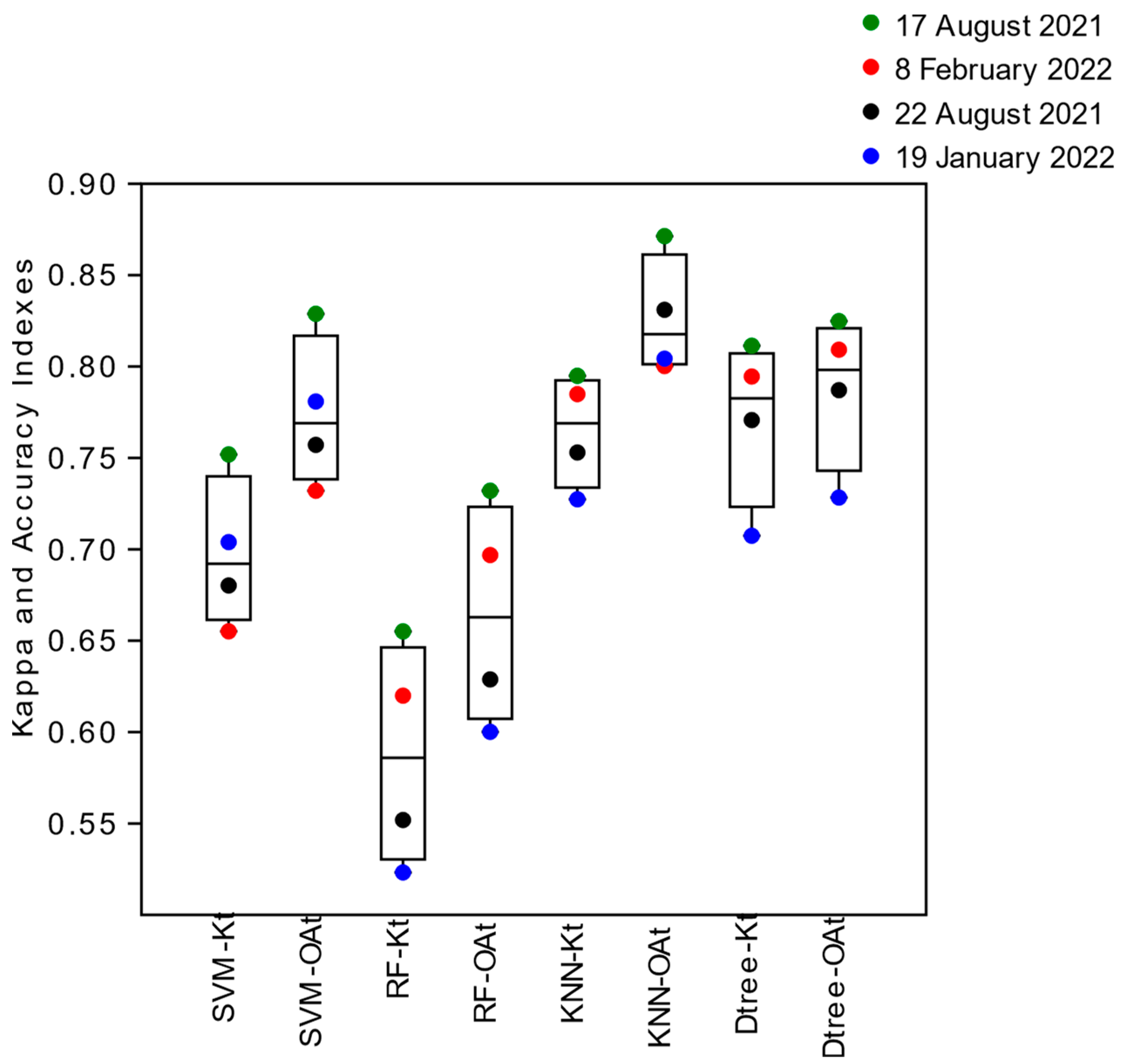
In another scenario, the Global Kappa Indexes (Kt) obtained by the algorithms (SVM, Random Forest, KNN, and Decision Tree) that had the entire segments in each image as training samples, were shown to be approximate for the images from 17 August 2021 (͞x = 0.75, sd = 0.07) and 8 February 2022 (͞x = 0.71, sd = 0.09), referring to the summer and winter season in quadrature conditions (lower tidal amplitude), and for the image from 22 August 2021 (͞x = 0.69, sd = 0.1) of spring tide (greater tidal amplitude) in summer, and more distant from the image from 19 January 2022 (͞x = 0.58, sd = 0.08) obtained in spring tide in the winter season (Figure 8). The algorithms that maintained the highest Global Kappa (Kt) Indices in the training of the classifiers in all images were KNN (͞x = 0.77, sd = 0.03) and Decision Tree (͞x = 0.77, sd = 0.05), and the smallest were the SVM (͞x = 0.70, sd = 0.04) and Random Forest (͞x = 0.59, sd = 0.06) (Figure 8).

The Overall Accuracy Indexes (OAt) obtained in the training of the algorithms, using entire segments as samples, demonstrated greater accuracy for the images of the summer season under neap tide conditions, 17 August 2021 (͞x = 0.81, sd = 0.06), and winter, 8 February 2022 (͞x = 0.76, sd = 0.05), and closer values for images obtained in spring tides in the summer season, 22 August 2021 (͞x = 0.75, sd = 0.09), and winter, 19 January 2022 (͞x = 0.73, sd = 0.09) (Figure 8). The algorithms that obtained the highest Overall Accuracy (OAt) Indices in the training phase were KNN (͞x = 0.83, sd = 0.03) and Decision Tree (͞x = 0.79, sd = 0.04), followed by SVM (͞x = 0.77, sd = 0.04) and Random Forest (͞x = 0.66, sd = 0.06) (Figure 8).

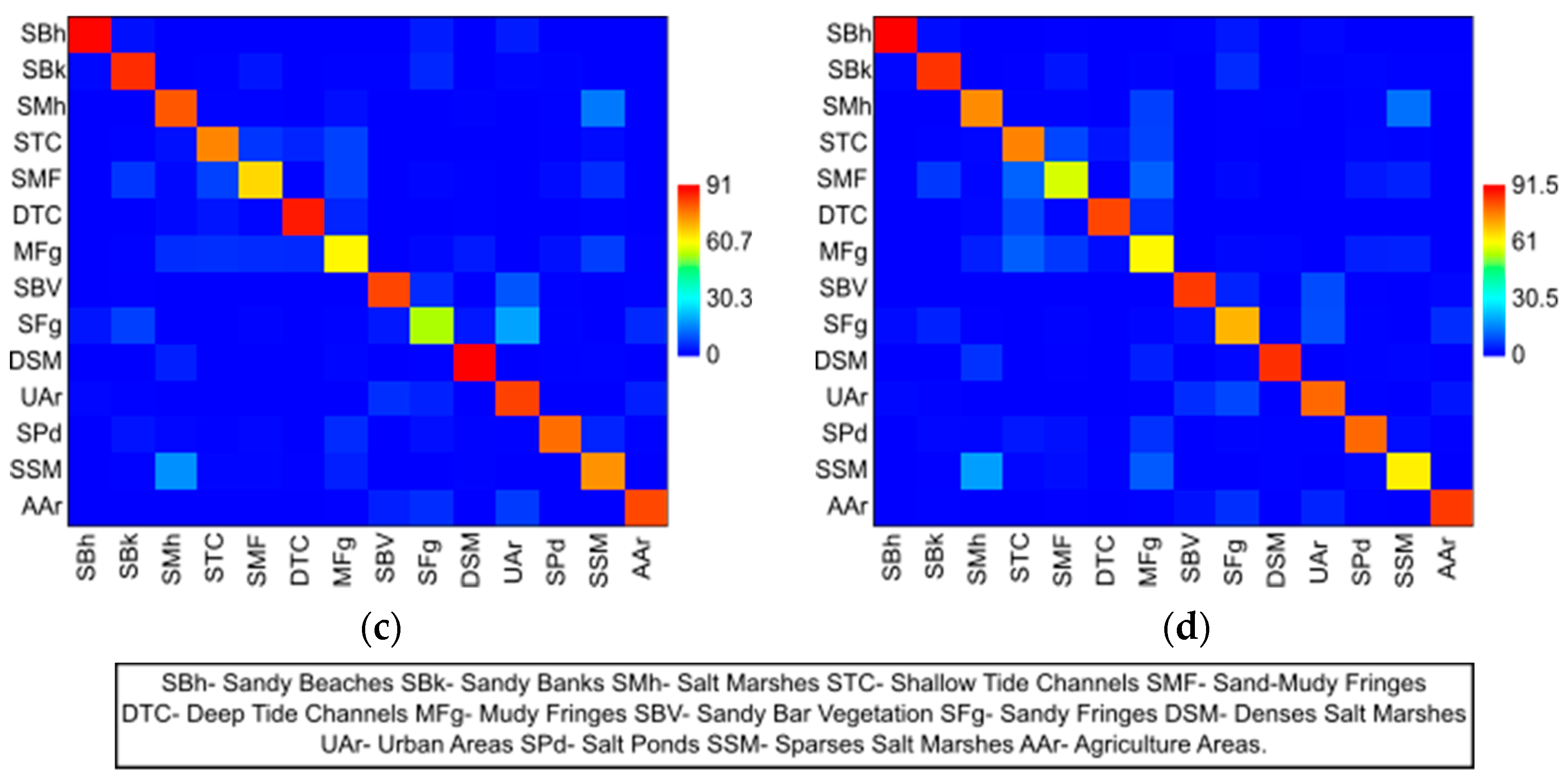
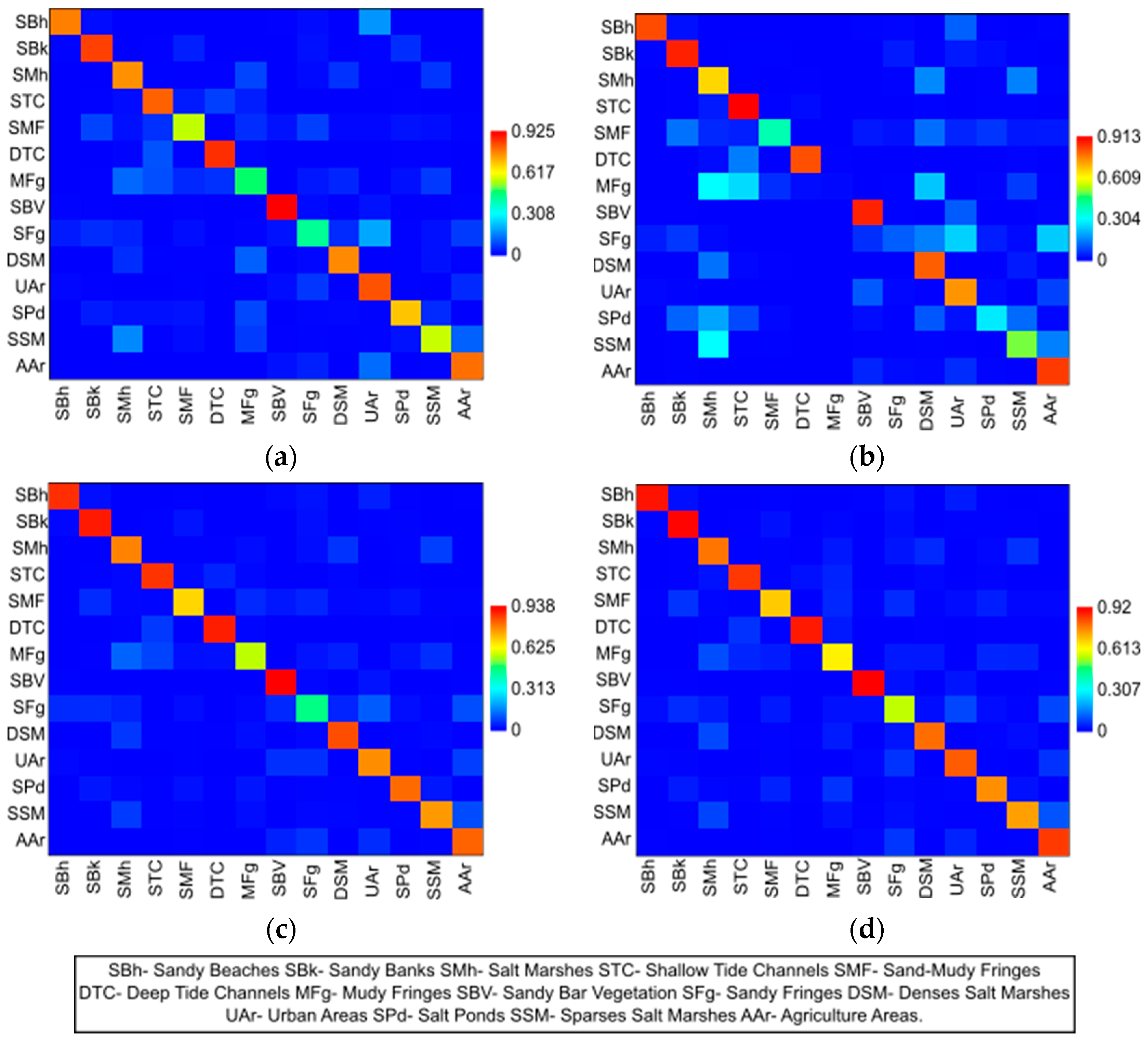
In the scenario in which the classifier algorithms used as training samples the polygons referring to the entire segments of each image, the confusion matrices showed that the SVM, KNN, and Decision Tree algorithms obtained the highest Recall (R) for the “Sandy Bar Vegetation” class (͞x = 0.92, sd = 0.04; ͞x = 0.94, sd = 0.02; and ͞x = 0.92, sd = 0.02, respectively). Random Forest obtained the highest Recall (R) for the “Shallow Tide Channel” class (͞x = 0.91, sd = 0.05). The Decision Tree obtained this for one more class, the “Sandy Bank” (͞x = 0.91, sd = 0.07) (Figure 9). The lowest Recall (R) values (on average “͞x” ranging from 0.45 to 0.11) were obtained by SVM, Random Forest, and KNN for the “Sandy Fringes” class, and SVM for the “Muddy Fringes” class, and by Random Forest for the “Sand-Muddy Fringes” and “Salt Ponds” classes (Figure 9).

In this same scenario, all classification algorithms obtained approximate Recall (R) values for the classes “Sandy Beaches”, “Sandy Banks”, “Salt Marsh”, “Shallow Tide Channels”, “Deep Tide Channels”, and “Agriculture Areas” (on average “͞x” ranging from 0.91 to 0.65) and more distant (on average “͞x” ranging from 0.81 to 0.28) for the “Salt Ponds” and “Sparse Salt Marshes” classes, with the highest values of Recall (R) obtained by KNN and Decision Tree, and the smallest by SVM and Random Forest (Figure 9).

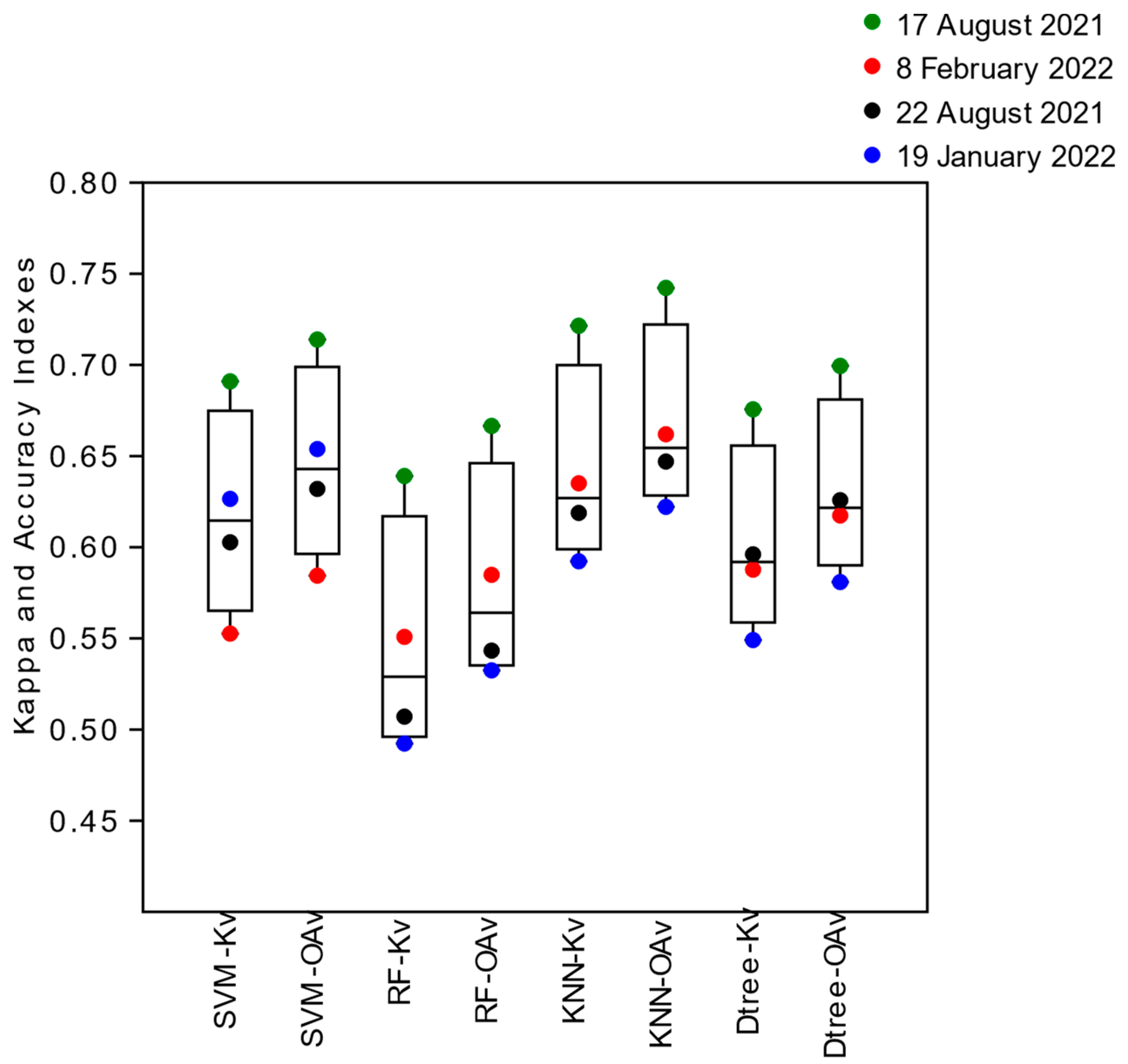
The Global Kappa Indices (Kv) obtained after validating the images classified by the algorithms (SVM, Random Forest, KNN, and Decision Tree), that had as training samples the entire polygons referring to the segmentation of each image, continued to show the highest indices for the images from 17 August 2021 (͞x = 0.68, sd = 0.05) and 8 February 2022 (͞x = 0.58, sd = 0.04), referring to the summer and winter season in quadrature conditions (lower amplitude of tide), followed by images from 22 August 2021 (͞x = 0.58, sd = 0.05) and 19 January 2022 (͞x = 0.57, sd = 0.06) obtained under spring tide conditions (greater tidal amplitude) (Figure 10). The algorithms that acquired the highest Global Kappa Indexes (Kv) after validating the image classification were KNN (͞x = 0.64, sd = 0.06), SVM (͞x = 0.62, sd = 0.06), and Decision Tree (͞x = 0.60, sd = 0.05). The lowest index was obtained by Random Forest (͞x = 0.56, sd = 0.07) (Figure 10).

The Overall Accuracy Indexes (OAv) obtained by validating the images classified by the algorithms, using as samples the polygons converted from the entire segments of each image, demonstrated greater accuracy for the images of the summer season in conditions of neap tides, 17 August 2021 (͞x = 0.71, sd = 0.03), and winter, 8 February 2022 (͞x = 0.61, sd = 0.04), followed by images under spring tide conditions obtained in the summer season on 22 August 2021 (͞x = 0.61, sd = 0.05), and winter on 19 January 2022 (͞x = 0.70, sd = 0.05) (Figure 10). The algorithms that obtained the highest validation Overall Accuracy (OAv) Indices were KNN (͞x = 0.67, Sd 0.05) and SVM (͞x = 0.65, sd = 0.05), followed by Decision Tree (͞x = 0.63, sd = 0.05) and Random Forest (͞x = 0.58, sd = 0.06) (Figure 10).

4. Discussion

As observed in this work, the image referring to 17 August 2021 obtained under the conditions of neap tide and summer season provided in the training (t) phase of the classification algorithms the largest (outliers) of the Global Kappa Indices (Kt) and Overall Accuracy (OAt), using both the samples of intersected segments and those of whole segments. The same was observed for this image about these indices in the image classification validation (v) phase (Figure 11).

The image of 17 August 2023, obtained under neap tide conditions and in the winter season in the training phase using samples from the intersected segments, according to the Kappa Index Scale of [21], obtained an almost perfect agreement (Global Kappa Index between 0.81 and 1.00) for the KNN and Decision Tree algorithms (Global Kappa Index = 0.82), and a substantial agreement (Global Kappa Index between 0.61 and 0.80) for the SVM and Random Forest algorithms (Global Kappa Index of 0.75 and 0.73, respectively) (Figure 11a). Furthermore, it was observed that the same agreements of the Global Kappa Index (Kt) in the training phase, using as samples the entire segments of each image, were maintained by the Decision Tree and SVM, but with smaller variation (−0.02) for the KNN, and higher (−0.07) for the Random Forest (Figure 11a).

The Global Kappa Indices (Kv) obtained in the validation phase of the classification of the image of 17 August 2021 by the algorithms remained approximate, being increased for the SVM when whole or total segments were used as a training sample (+0.03), and decreased for Random Forest (−0.03), KNN (−0.04), and Decision Tree (−0.06) (Figure 11b). Also, Ref. [22] reported that the Decision Tree was more sensitive to small changes in the training samples concerning the referred algorithms.

Ref. [3] observed that the SVM algorithm had a more significant impact on Overall Accuracy (OA) when trained with samples of more balanced pixel sizes between classes but with larger sample sizes. In this case, the image from 17 August 2021, obtained under neap tide conditions and in the winter season in the training phase using the intersected segments, better represented the samples for the Decision Tree, KNN, and Random Forest algorithms, except for the SVM (this was observed for the SVM algorithm, both by the Overall Accuracy (OAt) Indices in training (t), and validation (v) phase of the classification, increasing performance (by +0.06 and +0.02), respectively). In contrast, the other algorithms performed better with the intersected segments as training samples (Figure 11c,d). This pattern was held among the other images, except for the image from 8 February 2022 obtained under conditions of neap tide and winter season by Random Forest (+0.13 in training and +0.04 in validation), being more observed in the SVM algorithm (ranging from +0.06 to +0.15 in training and from +0.03 to +0.08 in validation) (Figure 11c,d).

The highest Global Kappa Indexes (K) and Overall Accuracy (OA) in the images from 17 August 2021 and 8 February 2022, obtained in summer and winter neap tide conditions, respectively, were related to the environmental conditions of slight tidal variation, in which the samples were better characterized by the classifier algorithms when the polygons intersected between the image segments were used as training samples, mainly in the summer season (17 August 2021). This was also due to the greater photosynthetic activity at this time of the year, which better detects the vegetation element and favors the detection of underwater features due to the greater light penetration into the water column. On the other hand, the images of spring tides were in environmental conditions of greater tidal currents, and, consequently, greater turbidity, which affected the characterization of samples of underwater features, reducing the Overall Accuracy of the classifiers under these conditions.

However, using the intersection segments between the images as training samples, these conditions were more minimized by the KNN and Decision Tree classifier algorithms than by the SVM and Random Forest algorithms in all images (Figure 11a,b). The KNN and Decision Tree classifiers, both in the training and classification validation phases, obtained substantial agreement (Kappa Index between 0.61 and 0.80) (Figure 11a,b). With this on the Kappa Index Scale by [21], the SVM and Random Forest algorithms obtained a substantial agreement in the training phase (Kappa Index between 0.61 and 0.80), but a moderate agreement (Kappa Index between 0.41 and 0.60) in the classification validation phase.

In another scenario referring to the training of algorithms using integer segments as a training exception, still according to the Kappa Index Scale by [21], the KNN and SVM classifiers both in the training phase and in the validation phase classification obtained a substantial agreement (Kappa Index between 0.61 and 0.80), while the Decision Tree algorithm obtained a considerable agreement in the training phase, but a moderate agreement (Kappa Index between 0.41 and 0.60) in the classification stage. In this condition, the Random Forest algorithm obtained a reasonable agreement in the classification’s training and validation phases (Figure 11a,b). The authors of [3] observed the same for the KNN algorithm when trained with a sample of greater numbers of pixels per class, under different size specifications and between courses of equal sizes.

The Overall Accuracy (OA) Indices obtained in the training phase as well as in the classification validation phase, using the sample with the segments intersected in training, have approached the values of the Kappa Index (more than +0.03), which according to [2], demonstrated that the number of validated pixels in all classes were proportionally distributed among the ranks, thus obtaining a more balanced or accurate classification performance between the algorithms (Figure 11c,d).

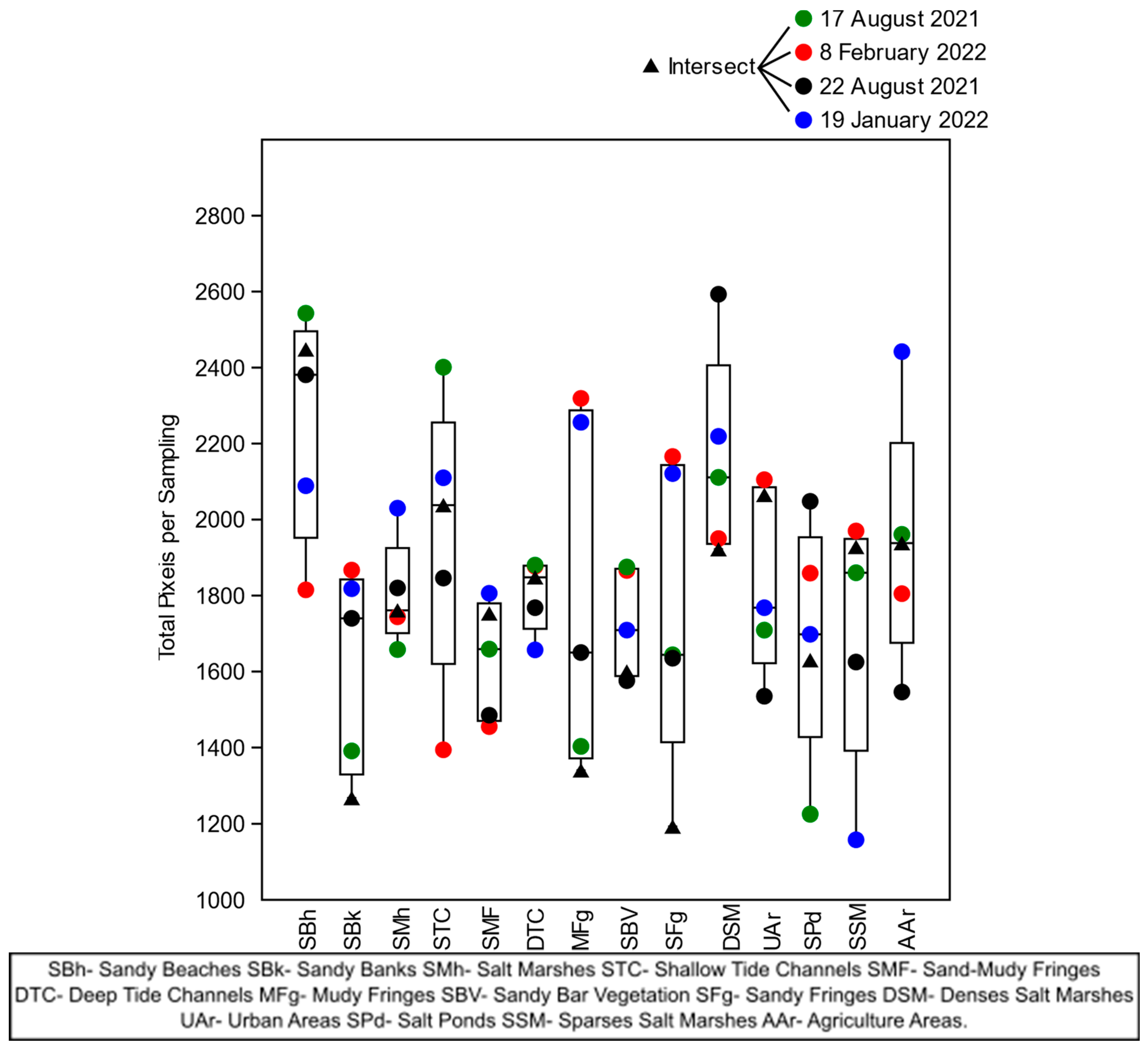
However, using integer segments as a training exception, training General Precision Indices were obtained (a majority of +0.08) relative to Kappa Indices, indicating the moderate variability between classes (Figure 11c,d). This effect was caused by the more significant variation in the size of the set of pixels in the training demonstrations when using the entire segments of each image concerning the intersected segments training demonstration (Figure 12), which may have increased the edge effect of the algorithm segmenter, generating a lower precision between the classes detected in the images. Unlike the others, the Random Forest algorithm, on average, was the one that obtained the most balanced results in the validation phases of training and classification (Figure 11b,d).

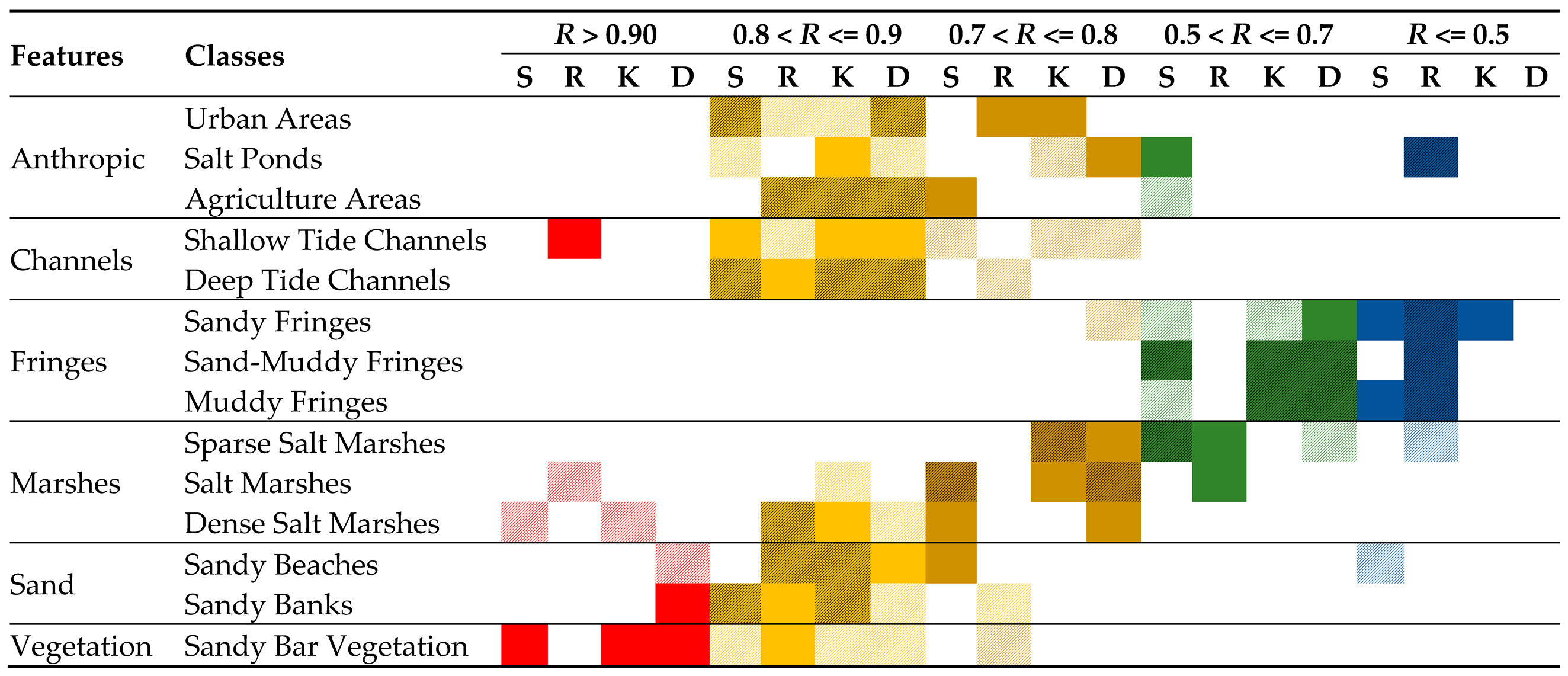
According to [20], the results of the Recall (R) measures obtained by the classifier algorithms, both in the scenario of using training samples using intersected segments and in the design of using entire segments, showed differences in the discrimination sensitivity of classes (

Table 2. Values of Recall (R) or True Positive Rate (TVP) obtained by the classifier algorithms SVM (S), Random Forest (R), KNN (K), and Decision Tree (D), using training samples from intersected segments (dashed cells), and entire segments (solid color cells).

). Excellent discrimination (Recall values > = 0.90) was obtained for the classes “Dense Salt Marshes” by the SVM and KNN algorithms, “Salt Marshes” by Random Forest, and “Sandy Beaches” by Decision Tree, using samples from the training of the intersected segments.

Otherwise, using the entire segment of each image as training samples, the “Sand Bar Vegetation” class achieved excellent discrimination by the SVM, KNN, and Decision Tree algorithms, as well as the “Shallow Tide Channels” class by Random Forest, and even the class “Sandy Banks” by Decision Tree (Table 2). In both training scenarios, the algorithms used demonstrated for these classes that the training samples were well segmented, characterized, and classified correctly from the respective spectral signatures between the bands of each image. Gradually on the Tharwat’s Discrimination Scale [20], of the 14 cover classes identified in the Ria Formosa in this study, most classes (10 classes) obtained from excellent to good discrimination among all the algorithms used (Table 2).

A good discrimination (Recall between 0.8 and 0.9) was met by the SVM algorithm when trained, both with the sample of the intersected segments and with the integers per image, for the classes “Sandy Banks”, “Deep Tide Channel”, and “Urban Areas”. In contrast, the classes “Sandy Bar Vegetation” and “Salt Ponds”, when trained with intersected samples, and “Shallow Tide Channel” with samples of entire segments, obtained a good description by the SVM classifier algorithm (Table 2).

The SVM addressed an acceptable discrimination (Recall between 0.7 and 0.8) for the “Salt Marshes” classes in the two sample usage scenarios and the “Shallow Tide Channel” class using intersected samples in the training. In another design, entire segments were used as an exception, such as the classes “Sandy Beaches”, “Dense Salt Marshes”, and “Agricultural Areas” (Table 2).

In the scenarios of using intersected samples for training as well as entire segments, the Random Forest algorithm demonstrated good discrimination (Recall between 0.8 and 0.9) for the classes “Sandy Beaches”, “Dense Salt Marshes”, and “Agriculture Areas”; and when using only the training samples of intersected segments, the classes “Shallow Tide Channel” and “Urban Areas” had good discrimination (Table 2). The same happened in the other scenario with the use of the entire segments for training for the “Sandy Banks”, “Deep Tide Channel”, and “Sandy Bar Vegetation” classes. These last classes passed in turn to acceptable discrimination (Recall between 0.7 and 0.8) when using the training samples that were the intersected segments, as well as the inverse for the class “Urban Areas” when the training was using the entire segments (Table 2).

The KNN classifier algorithm in all scenarios was the one that demonstrated good discrimination for more classes (10 classes) (Recall between 0.8 and 0.9) being, in this case, the classes in the two training scenarios, “Sandy Beaches”, “Sandy Banks”, “Deep Tide Channel”, and “Agriculture Areas”; and in training with samples of intersected segments for the classes “Salt Marshes”, “Sand Bar Vegetation”, and “Urban Areas”, and in training with the use of the entire segments, the classes “Shallow Tide Channel”, “Dense Salt Marshes”, and “Salt Ponds” (Table 2). Acceptable discrimination (Recall between 0.7 and 0.8) was obtained by KNN in the two training scenarios only for the “Sparse Salt Marshes” class and in the scenario using intersected samples for the “Shallow Tide Channel” and “Salt Ponds” classes, as well as for the “Salt Marshes” and “Urban Areas” classes in the scenario of using samples of entire segments for training (Table 2).

The Decision Tree classifier algorithm in both training scenarios obtained good discrimination (Recall between 0.8 and 0.9) for the classes “Deep Tide Channel”, “Urban Areas”, and “Agriculture Areas” (Table 2). This was also true for the “Sandy Banks”, “Sandy Bar Vegetation”, “Dense Salt Marshes”, and “Salt Ponds” classes, in the training scenario using intersected samples, and for the “Sandy Beaches” and “Shallow Tide Channels” classes in the training scenario using samples with whole segments per image (Table 2). Acceptable discrimination (Recall between 0.7 and 0.8) was obtained by the Decision Tree classifier algorithm only for the “Salt Marsh” class; in training, the scenario using intersected samples for the “Shallow Tide Channel” and “Sandy Fringes” classes; and in another scenario of samples of entire segments, for the classes “Dense Salt Marshes”, “Salt Ponds”, and “Sparse Salt Marshes” (Table 2).

The Ria Formosa land cover classes, referring to the fringes of the “Sandy Fringes”, “Muddy Fringes”, and “Sand-Muddy Fringes” channels, and one of the “Sparse Salt Marshes”, were obtained by the SVM and Random Forest algorithms in both training scenarios, according to the Tharwat’s Discrimination Scale [20], weak discrimination, as well as not being discriminated (Table 2). These classes in all images represented areas with a more significant effect on tidal dynamics and seasonality. These varied daily due to hourly flooding, allowing mixtures of spectral responses from the terrestrial, subaqueous, and aqueous environments.

The classes obtained by SVM with weak discrimination (Recall between 0.5 and 0.7) in both training scenarios were “Sand-Muddy Fringes” and “Sparse Salt Marshes”, and with the use of the intersected samples, were “Sandy Fringes”, “Muddy Fringes”, “Sand-Muddy Fringes”, and “Agriculture Areas”. In the scenario of using samples of entire segments per image, there was only the “Salt Pond” class (Table 2). Classes without discriminative power (Recall < = 0.5) were also obtained by SVM, with the “Sandy Beaches” class due to being strongly confused with the “Urban Areas” class by training with intersected samples (Table 2 and Figure 6a). In the other scenario of using samples of entire segments of each image, the classes “Muddy Fringes” and “Sandy Fringes” had no discriminative power (Table 2).

Weak discrimination (Recall between 0.5 and 0.7) was obtained by the Random Forest classifier algorithm only when trained with the entire segments of each image for the “Salt Marshes” and “Sparse Salt Marshes” classes. On the other hand, the classes without discriminative power (Recall < = 0.5) were higher for this algorithm (five classes), being in both training scenarios, and referring to the fringe classes of the channels “Sandy Fringes”, “Sand-Muddy fringes” and “Muddy fringes”, and even “Salt Ponds”, as well as the use of the intersected segments for training for the “Sparse Salt Marshes” class (Table 2).

The KNN and Decision Tree classifier algorithms obtained weak discrimination (Recall between 0.5 and 0.7) in both training scenarios for the “Sand-Muddy Fringes” and “Muddy Fringes” classes, with KNN for the “Sandy Fringes” class and the Decision Tree for the class “Sparse Salt Marshes”. There was weak discrimination when using samples of intersected segments for training (Table 2), and still, weak discrimination by the Decision Tree for the class “Sandy Fringes” when using samples of entire segments for training (Table 2).

Both the KNN and Decision Tree algorithms did not obtain classes without discriminative power (Recall < = 0.5), with the use of training samples being those of intersected segments, but it was obtained by KNN, for the “Sandy Fringe” class, by using samples that were those of whole segments for training (Table 2).

Considering only the merge of classified images (overlapping and applying a majority filter) after the classified images were recoded to exclude classes that had no discriminative power (Recall < = 0.5), the Global Kappa Indexes and the General Accuracy Indexes, after the validation, were better for classified fused images trained with intersected segments (

Table 3. Comparison of the Global Kappa Index (k) and the Overall Accuracy Index (OA) obtained after validating the fused and non-fused classified images trained with samples of intersected and entire segments.

Classified Image	Samples of Intersected Segments				Samples of Entire Segments
	Non-Fused		Fused		Non-Fused		Fused
	k	OA	k	OA	k	OA	k	OA
8 February 2022	0.60	0.63	0.72	0.74	0.58	0.61	0.70	0.72
17 August 2021	0.71	0.73	0.80	0.81	0.68	0.71	0.78	0.79
19 January 2022	0.58	0.61	0.71	0.73	0.57	0.60	0.68	0.71
22 August 2021	0.59	0.62	0.68	0.71	0.58	0.61	0.68	0.71

). Also, the application of the fusion of the classified images in both training scenarios allowed the increase in the Kappa Indexes and the Overall Accuracy of about 10% concerning the non-fused classified images (Table 3).

Taking into account the cost–benefit evaluation of the use of traditional ML algorithms, which generally provide an accuracy between 80% and 90%, using a smaller number of classes of use and occupancy, this work obtained an accuracy between 71% and 81%, achieved by merging images classified by ML algorithms such as SVM, Random Forest, KNN, and Decision Tree, for 14 classes of use and occupation of the Ria Formosa (Table 3).

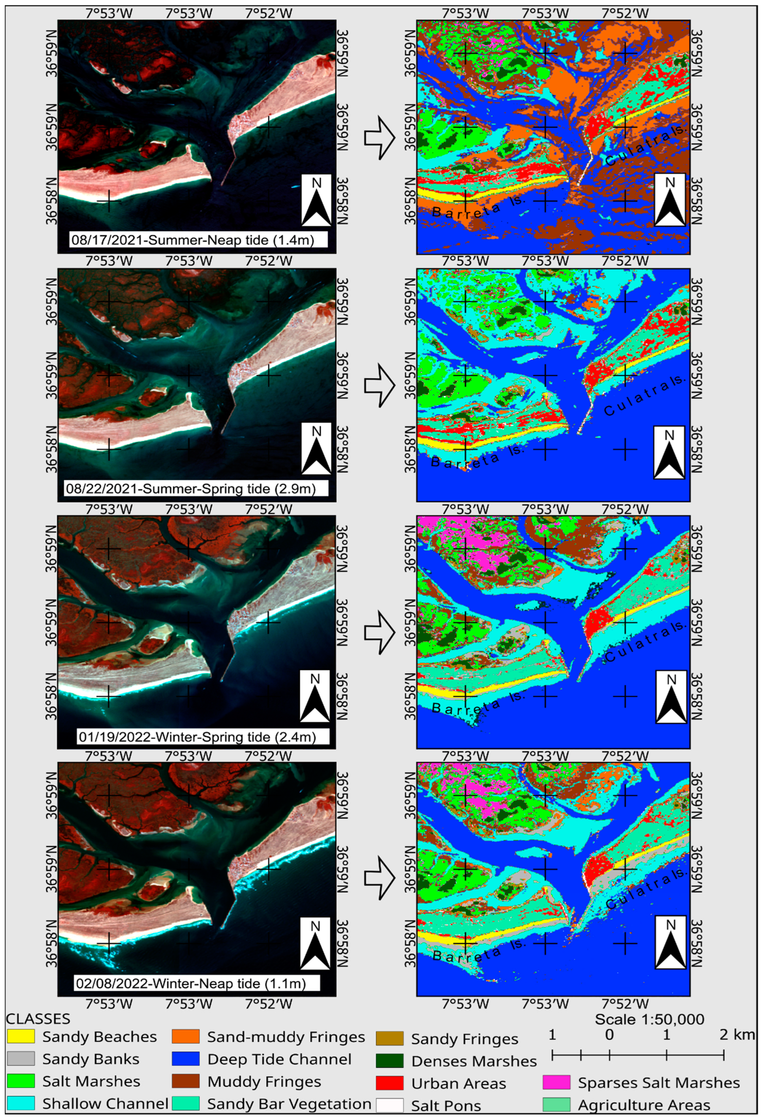
Analyzing the time series of the images in a section of the area in the channel between Barreta and Culatra Islands (Figure 13), it was possible to verify that the classes obtained by merging the classifiers referring to the image from 17 August 2021 (summer and mare quadrature) were more diverse due to the detection of underwater features such as channel fringes, sandbars, and bottom facies. Also, the merger of the classifications was observed in the image from 22 August 2021 (summer and spring tide). However, fewer classes were obtained in that portion, reflecting the dynamics of the channels (shallow and deep) that surround the islands and marshes, such as areas of flooded marshy vegetation, in addition, of course, to beach strips (in yellow) and urbanized areas (in red) most used during the summer on the islands of Barreta and Culatra (Figure 13). These classes contributed with great potential for the characterization and monitoring of hydrodynamics and coastal sedimentation.

In the Winter Station, in the images from 19 January 2022 (spring tide) and 8 February 2022 (neap tide), it was possible to observe the increase in sparse swampy areas (in magenta) due to the decrease in the photosynthetic activity of the vegetation marshland, different from sandbank vegetation (light green-blue) which expanded due to the decline in anthropic activity (in red). Also, in the image from 8 February 2022 (neap tide), there was a greater formation of sand banks (in gray) parallel to the beaches due to the period of the greater incidence of waves (Figure 13).

5. Conclusions

In this work, we present the results of a multiclass classification problem with 14 classes of forms and land use and occupation. The image multiclass classification was computed using four different machine learning algorithms: SVM, Decision Tree, KNN, and Random Forest, and four image datasets from Sentinel 2 satellites. The images were collected in summer (two datasets) and in winter (two datasets) with different tide stages, considering the great diversity of ecological conditions of the study area.

For the training of the machine learning algorithms, there were five vectorial datasets with polygons for georeferentiation of the considered classes. There was one vectorial dataset for each image dataset, plus one obtained from the previous one obtained by spatial intersection of the polygons of the same class. The results in the validation phases show that this last one (segments intersected) can be used to build the input to train and test the algorithm for each image dataset with similar levels of accuracy.

This work used a more significant number of classes (14) to be discriminated by the algorithms SVM, Random Forest, KNN, and Decision Tree; 10 categories were well distinguished. The few discriminated classes referred to the features of fringes or edges of channels, which were confused due to the different variations or mixtures of sand and mud, suggesting that this work tested a more significant number of classes for these algorithms than other works and that it pointed to the need to look for classifier algorithms with greater sensitivity, or Recall (R), to these feature variations; the same was true to carry out different sampling strategies for training that have this detection capability.

The classification algorithms that obtained greater accuracy using the training samples with the segments intersected between the images were KNN (͞x = 0.71, sd = 0.05), Decision Tree (͞x = 0.68, sd = 0.05), SVM (͞x = 0.61, sd = 0.05), and Random Forest (͞x = 0.59, sd = 0.08). Otherwise, those using entire segments as training samples were KNN (͞x = 0.67, sd = 0.05), SVM (͞x = 0.65, sd = 0.05), Decision Tree (͞x = 0.63, sd = 0.05), and Random Forest (͞x = 0.58, sd = 0.06). However, Random Forest was not more accurate than Decision Tree but was a more balanced algorithm in two scenarios of training.

Despite obtaining an accuracy greater than 81% in this work, using a joint approach given by the fusion of the SVM, Random Forest, KNN, and Decision Tree algorithms, it is still possible to propose the evaluation of the use of neuronal ML algorithms. These algorithms, although they will require more adjustments of hyperparameters, can still be examined in the sense of obtaining a greater accuracy of classification, as, recently, the application of algorithms that simulate neural networks has been taking place in the sense that they assign weights to the connections that best characterize the nature of the input data.

This work also pointed to intersecting the segments within the images in a time series, as more balanced results were obtained between training accuracy and validation. At the same time, it constituted more representative samples of the classes to be identified in the images by the classification algorithms, which can be used to implement monitoring tools by satellite image to obtain an accuracy between 80 and 90% of mapping.

As noted, the use of Sentinel 2A/2B images in the context of image classification by ML algorithms has excellent potential for the characterization and environmental monitoring of areas of intense and complex environmental dynamics, such as the Barriers Islands System of Ria Formosa, thus demonstrating that it is possible to use these algorithms as a monitoring tool that is easy to implement in GIS. Therefore, this is becoming an advantage compared to the more traditional forms of implementation of unsupervised and supervised classification algorithms used in GIS, which reach a general accuracy of 60 to 70%, with more steps and still similar operational costs of ML used in this work.

An accurate database of classes of environmental, economic, and infrastructure resources can help researchers in several areas due to the potential it has to make it possible, for example, to assess more coherently scenarios of agricultural production, growth of the urban regions, deforestation and fires, and erosion processes, among other environmental impacts.